Part II – Not Out Innings and Batting Averages – Demystifying Rarefied Solutions & a Searchlight on the Straightforward

Peter Kettle | 9:56am GMT 30 January 2022

PART II – THE STRAIGHTFORWARD SCHOOL

No doubt there have been many types of straightforward solution devised by those participating in cricket forums and other informal settings. Yet, in published form, such solutions are few. During a conscientious search I unearthed just four of them, all originating in the new millennium. Three of these proposals revolve around a common basic theme, but with important differences.

Initially, though, some comments are in order on two simple solutions. They are briefly discussed in an article of 2014 by Kartikeya Date, who is a frequent writer in various forums on topical cricket matters. What he goes on to advocate is replacing the Traditional Average by the average score of all innings (completed and Not Out) that lie within the range of 0 to 100 runs. This is directed to combining batting “quality and consistency”, and is proposed as it “accounts for events that occur frequently while the traditional measure is disproportionately affected by events that occur only rarely”.

Although this proposed statistic (which Date labels “the score”) strays into different territory than this essay, at root is the simple number of runs scored per innings played. That particular measure hasn’t caught on as a replacement for the Traditional Average (as distinct from being an interesting complementary notion), probably because it denies batsmen what might be called their rightful entitlements. But, as he notes, if the upper limit for his own proposal is set high enough (at 400 runs, instead of a cap at 100), it would boil down to number of runs scored per innings played. This, I think, would be a lot more palatable to specialist batsmen than his capped proposal. Yet even that version would be unsuitable for those making a relatively high proportion of Not Out scores, chiefly those of the lower middle order and tail.

The other simple measure that Date mentions is the Median Score – ie the middle value of all the scores a batsman makes. This turns out to be a lot lower than the Traditional Average (TA). For the Test career of Brian Lara, the Median Score is 33.5 for all innings and 33.0 excluding Not Outs (TA of 52.88); for Steve Waugh the corresponding figures are 25.5 and 20.0 (TA of 51.06); and for Mohinder Amarnath the figures are 30.0 in both cases (TA of 42.50). Whilst the relativities so produced for these three specialist batsmen might be thought reasonable, the Median Scores given are heavily influenced by failures occurring during the playing-in phase of an innings. And it is during that phase that good and bad luck play a large role in determining whether or not a batsman survives to become well established.

Having disposed of these two possible measures, I turn to consider the main straightforward contributions in chronological order. The first is a method of deriving batting averages that is implied by the Melbourne-based statistician Charles Davis. It is contained in his book, The Best of The Best (published in year 2000) when discussing a myth about the general impact of Not Out Innings on Traditional Averages (pages 96-98). Whilst his favoured method of handling Not Out Scores is not directly stated, it has been detected by closely examining the relevant parts of his text.

Davis’ graph (page 97) shows an estimate of the additional runs that a batsman will add as he reaches successively higher scores in an ultimately completed innings, which ranges from the start of an innings (on zero) through to when on a score of 255 (for those who have survived that long). The data reflect the performance of the overall careers of past and present Test players.

Charles Davis – first of the Straightforwards

Substituting career data on an individual batsman for Davis’ generalised batsman (or generality of batsmen), such a graph can be used to indicate what that batsman would, potentially, have gone on to add to his score if not forced to retire Not Out (though Davis himself doesn’t highlight this point). Hence, it can be used to make predictions of the likely outcome of a given Not Out Score for any particular batsman. 

The number of runs typically added by Test batsmen after being on a specified undefeated score is presented by Davis in terms of both a Mean and a Median value. He favours using the set of Median values as the being a better indicator of “most likely outcomes” – that is, of the additional runs expected to be made.

The second straightforward proposal emanates from Uday Damodaran, now a Professor at the Indian Institute of Management at Udaipur (north-west India). This is outlined in his article of 2006. The proposal itself forms an input to his study of ODI batting performance by the Indian team and takes up just one of the article’s four pages. In similar fashion to Davis, but explicitly laid out, a Not Out Score is projected to a notional conclusion.

The number of runs that a Not Out player could, potentially, have gone on to score – had he been able to bat on – is made dependent on the outcomes of the series of innings played previously. The number of runs the batsman would likely have ended up scoring is given by the Mean value (ie the arithmetic average) of each of his prior innings which made a score greater than or equal to the Not Out Score in question. In effect, the relevant prior scores are simply added up and divided by the number of innings played – which is in contrast to Davis’ preference for taking the Median value.

These prior scores are, in effect, all given an equal probability of reoccurring:

For example: three individual scores of eighteen runs are each given the same probability as a single score of, say, twenty runs and so the former are counted three times. If the total number of relevant innings is 40, these four individual scores would each be accorded a probability of (1/40) 0.025.

Matters stop there. All information that becomes available about the batsman’s performance after the Not Out Innings (NOI) in question is ignored, unlike with Davis who has regard to all innings a batsman plays during his career. Damodaran considers that his statistic provides a good estimate of the number of additional runs in effect denied to the Not Out batsman concerned.

A brief digression on terminology: if the expectation of a potential outcome occurring is based on known outcomes that have already occurred, as with Damodaran’s solution, it is referred to in the literature as a conditional probability. And so the estimated score that a batsman would have gone on to make is termed his conditional average at that point in time, given he has already scored a certain number of runs before having to retire Not Out.

Damodaran refers to his approach as Bayesian because what is considered the most probable completion score for a Not Out Innings (NOI) depends on knowledge of events as they unfold. Hence, at the time a given NOI occurs, the prediction of the likely completed score is based on those events (innings) taking place previously. And, as the batsman’s career progresses, account is taken of the additional innings played prior to the next NOI occurring, and so on.

This label is in recognition of Thomas Bayes, an English statistician (living from 1701-61), whose methodologies were further developed by Pierre-Simon Laplace from the late-18th to the early-19th century. The central feature is that a belief, or hypothesis, held about the likelihood of an event occurring is updated as further information (or evidence) becomes available – in our case, the updating of a batsman’s conditional average.

A separate point is that intuition tells us that a batsman having to retire Not Out might have made any possible score within the range of those previous scores made that equal/exceed his score on retiring. So why not take the average of all these possibilities, even though he didn’t actually end up making some of them? The snag with this solution is that the spread of scores he does make may be substantially uneven, and likely with a high proportion of them being terminated during the fraught playing-in phase. So the actual distribution of the scores made is important, and filling in between them to give a continuous string of scores may often be misleading.

Assigning each relevant score made an equal probability of being reached, had he batted on, is obviously a simplifying assumption – ignoring, as it does, factors such as the quality of the opposition bowling, the pitch condition and distance of boundaries from the wickets. These sort of factors could be assessed, and predictions of the likely completed score made responsive to them, but this would tend to be over-demanding of the available information. There would usually be an insufficient number of scores made in different circumstances to enable reliable results to be produced.

Damodaran’s projected Not Out Scores (NOSs) are included along with all actually completed innings, before dividing through by the number of innings played so as to establish the batsman’s “true” average. The ODI careers of 14 batsmen are included in his analysis. The recommended procedure is illustrated for Sachin Tendulkar’s initial 15 ODI innings, which contains two NOSs.

A refinement he makes on Davis’ approach is that any other NOS (occurring prior to the NOS in question) is potentially included in the series to be averaged at its projected-to-completion value, depending on whether this equals/exceeds the NOS in question.

Although Damodaran gives a clear illustration of his procedure in operation, it is a pity that he doesn’t provide any examples of what the resulting batting averages are for comparison with their traditional counterparts.

More recently, Paul Ulrick – a member of the UK based Association of Cricket Statisticians – has derived an adjusted set of averages in an article of 2020. He presents a well-rounded, and fullish account of what he did and why, and also details the results of applying his proposal to the careers of 52 Test players (selected from a pool of 550).

His treatment differs from that of Damodaran in two important respects. First, Ulrick’s projection of a given NOS to a likely conclusion is based on all those equal and higher Dismissal Scores made throughout a batsman’s entire career, rather than on only those occurring prior to the NOS at hand. As he puts it, the relevant scores for projection are identified “irrespective of at what stage during the batsman’s career the not out innings in question has occurred”. In practical terms, this is a merit in my view (as discussed shortly), although Ulrick doesn’t give a related reason for his choice.

The second main difference is that, in projecting a NOI, whereas Damodaran factors in projections made for other (prior) NOSs, Ulrick limits consideration of relevant scores to those made from dismissal innings only. This is an unnecessary restriction, and it somewhat reduces the value of his findings.

Ulrick flags the problematic case in which a batsman’s highest career score comes from a NOI, saying that “intervention is required”. Although he doesn’t pursue this matter in discussion, in his calculations Ulrick has treated this in the traditional way, as an expedient – letting the score stand as it is and not counting it in the denominator (number of innings actually and notionally completed). This is how he deals with Gary Sobers’ undefeated innings of 365 (made against Pakistan at Kingston in February 1958).[i]

The theme of Ulrick’s article is how the tension between a denied opportunity to advance a score and possible imminent demise plays out for Not Out innings. For his sample of 52 Test batsmen, mostly with more than 1,000 runs to their name, the overall finding is: “except for a few extreme cases, the positive impact that Not Outs have on the traditional average is largely offset by the opportunity to achieve a larger score”.

In only 9 of the 52 cases does the Adjusted Average exceed the Traditional Average and all of these are by less than 2%. In 16 of the 43 cases of a decrease on the Traditional Average, this is very small (less than 1%).  However, in 13 cases – including all five of the tail-enders in the sample – the decrease is at least 5%. These thirteen players all had a high proportion of their runs coming from Not Out Innings – 30% and upwards. Ulrick finds that, predominantly, the higher the proportion of runs coming from Not Out Innings, the greater is the percentage difference between the Adjusted and Traditional Average. These two factors are strongly correlated.

The comparison just made of Damodaran and Ulrick’s respective methods raises two general issues. On the first issue of whether to have regard to a batsman’s overall career or only those innings played prior to a Not Out Innings to be projected, there are arguments in favour of both their choices. The case for taking a whole career approach is as follows. The course that batsmen’s careers generally take is of making relatively low scores initially, followed by a considerably longer period of moderate to high scores when being established, after which there is a declining trend as the player’s aging exerts an increasing influence.

So, ideally one would like to divide up the analysis into these three career phases. This way a Not Out Score (NOS) made in the initial period would be projected on the basis of relevant scores made during that period alone and hence would not be artificially boosted by the better scoring of the middle period. Yet this would encounter many complications of how exactly to make the divisions, and how to treat batsmen who don’t more or less conform. Taking the whole of career perspective appears to have the greater merit for practical application. Therefore, “retrospective” prediction is admissible, and indeed desirable, in light of this point about the difficulty of tailoring estimates to a career’s different phases.

Secondly, as noted, both Damodaran and Ulrick apply the Mean value (ie the arithmetic average) of relevant scores as the guide to the likely conclusion of each Not Out Innings (NOI) and hence the additional potential runs involved. As now explained, in general this constitutes a drawback.

The issue is one of how representative either of the two measures – the Mean value and the Median value – is for predictive purposes. This question may be a second order one, but it is of some importance. Batting scores are rarely highly symmetrical – that is, with approximately the same number of scores either side of the Mean score, and with the Mean and Median scores being close together. Instead, the distribution of scores tends to be skewed to some extent. The presence of significant skewness is evident from an obvious change in the slope of the progression of scores, moving from high to low (or vice versa). In turn, the relevant scores for projecting a given NOS to an expected completion (ie those scores equal to and above it) may also tend to be somewhat skewed – depending on the segment of the overall distribution concerned.

To elaborate: when the degree of skewness of scores for projecting a NOS is only mild (according to a standard statistical test), the difference in the resulting projected score from using the two measures – Mean and Median value – will be small, and the impact of applying one or the other for the resulting “true” average will usually be immaterial. But when a test shows the relevant data on scores to be either moderately or highly skewed, as it often is, the Mean value will be both unreliable for predicting the conclusion of a NOS and tend to give a misleading estimate of the “true” overall average. In these cases, the Median value should always be used.

Hence, the Median value will usually be a better guide as to the most likely outcome – ie the potentially completed score. This view is consistent with the advice of Charles Davis, noted earlier, which reflects mainstream thinking. The Mean will be the best indicator of the likely outcome of a NOS only in certain special cases, which are only rarely encountered. The most frequent score, the Modal value, is very rarely a suitable indicator.

It has also been formally demonstrated, for instance in the article by Melinda Holt and Stephen Scariano (2009), that in a decision context with a skewed set of observations, applying the Median value is better than the Mean (or the Modal) value for minimising the absolute magnitude of the prediction error.

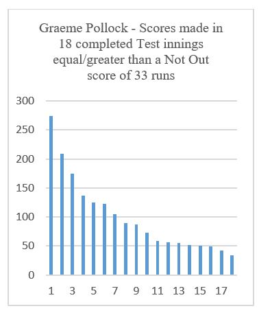
Examples of moderately skewed distributions of batting scores are shown below for Gary Sobers and Graeme Pollock in Test matches, both being included in Ulrick’s sample and his reported results.[ii] In both cases, the Mean value of the distribution is considerably higher than the Median (which is, by definition, always at the mid-way position of the data), which is caused by the fairly steep rise in the high end of the scoring series. For Sobers, the Mean value is a score of 52.6 runs and the Median value is 41.0; for Pollock, the Mean is 99.7 and the Median 80.0.

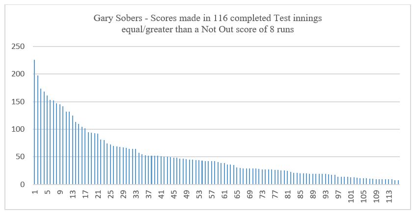
The impact that a skewed distribution of a batsman’s scores has on the resulting estimate of his “true” average depends on both the degree of skewness that the data exhibits and the proportion of innings that are Not Out. A high degree of skewness may have little impact on the estimated “true” average if Not Outs are a small proportion of all innings played.

For some of Ulrick’s selected batsmen, appreciably different results arise from applying the Median rather than the Mean value of relevant scores for projecting NOSs. In the case of Graeme Pollock, an increase on the Traditional Average of 1.6% would be turned into a reduction of 1.3%; for Gary Sobers, a reduction of 3.2% would grow to become 5.3%; and for Steve Waugh a reduction of 5.0% would grow to become 8.5%.

In fairness to Ulrick, he states that the work is of a preliminary nature, and so perhaps he regards application of the Median value as a potential refinement for the future. In respect of Damodaran, the scores of Tendulkar for his 336 completed ODI innings (up to the cut-off date) exhibit only mild skewness and, for practical purposes, use of the Mean value would be just as suitable as the Median. This point also applies to his illustrative example of Tendulkar’s initial 15 innings: each of the two Not Out scores have prior completed scores of equal/greater magnitude that are not significantly skewed. And Damodaran doesn’t explicitly rule out use of the Median value for some, or all, of the other 13 players analysed.

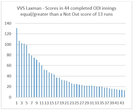
A highly skewed distribution of scores applies, for example, to VVS Laxman, being one of these other players – as shown below (Mean score of 41.9, Median score of 27.5).[iii]

Some readers might regard all of the combinations noted above for projecting Not Out Scores to a conclusion as being inadequate because they have no regard to the circumstances surrounding the scores on which the projections are based. Whilst desirable in principle, it would be over-ambitious to attempt to do so with reference to the context of the match and the innings concerned: such as the quality of the opposition bowling and who the batsman would be facing if continuing on, the state of the pitch and distance of boundaries from the middle. This would be too demanding of available information, unless analysis is limited to future events which would require an agreed methodology to give consistency of treatment. And the work entailed in operating it for all First Class players would be very considerable.

Turning, lastly, to the method advocated by Anantha Narayanan,a frequent contributor of discussion pieces in a number of forums. This goes by the name of The Weighted Batting Average. It is similar in spirit to the exposure to risk approach reviewed in Part I, and is based on runs scored rather than number of deliveries faced. Narayanan advocates his method with much conviction. Whilst having its origins nearly a decade ago, in its current form it is explained, with illustrative applications, on the Cricinfo website in an article of August 2021.

The Weighted Average for a batsman is estimated in four steps:

(i) All Dismissals, irrespective of the score made, are assigned an innings count of 1.0 (ie a weighting of 1.0).

(ii) All Not Out Innings with scores above the batsman’s Average Runs per Dismissal (ARD) are also assigned an innings count of 1.0.

(iii) All Not Out Innings with scores equal to or below the ARD are assigned proportional innings values between 0.0 and 1.0, the value in each case depending on the particular score made. (In effect, the various Not Out Scores are added together and then divided by the ARD to convert them into a number of completed innings equivalents.)

(iv) The weightings assigned are then added – which might give a total of, say, 33.5 which would then represent 33.5 (actually and notionally) completed innings.

The various scores in the above three categories all stand as they are in numerical terms, unaltered. The sum of the scores is divided by the total number of innings so derived which gives the Weighted Batting Average. This is, inevitably, always lower than the Traditional Average.

The principal point of note is as follows. If a Not Out Innings (NOI) falls into the second category, it is treated as though it is completed. If it falls into the third category, it is treated as a fraction of a completed innings, being valued pro rata to the batsman’s average number of runs for his Dismissal Innings. In both cases, the batsman is not credited with any further potential runs. This is obviously harsh.

Narayanan’s rationale for this approach is highly pragmatic as well as being very brief. It is stated as a compromise between, on the one hand, the Traditional Average – which is viewed as “intrinsically unfair to batsmen with a low proportion of Not Outs” – and, on the other hand, the most simple of all forms, being the “plain-vanilla runs per innings played” with no distinction being made between uncompleted and completed innings which “would swing the pendulum the other way…What is needed is something in the middle – logical, fair and accurate.”

Having applied his recommended procedure to many Test batsmen, Narayanan reports that the ratio of Weighted Batting Average to the Traditional Average ranges from 100% for two batsmen with zero NOIs (Marnus Labuschagne and Kaushal Silva) through to 78% for Shaun Pollock (with 25.5% NOIs).

The results are given for six Test batsmen. The largest proportional reductions on the Traditional Average are incurred by those with the highest percent of NOIs:

• Andy Flower and Steve Waugh, respectively with reductions of 14.1% and 14.6%, associated with 17.0% and 17.7% of NOIs.

At the other end are:

• Brian Lara and Saeed Anwar, respectively with reductions of 2.9% and 2.2%, associated with 2.6% and 2.2% of NOIs.
  
• About mid-way between these four sit Sachin Tendulkar and Herbert Sutcliffe.[iv]

Narayanan defends the resulting adjustment to the Traditional Averages for these six exemplars as being “very fair and equitable…the maximum benefits accrue to those batsmen with fewer Not Outs (as a proportion of all innings played). Those with a high proportion of Not Outs do not lose out – rather, they do not gain in an undeserved manner, as was happening with the traditional average. The WBA value is always lower than the traditional average. The relevant factor is the extent of drop.”

						% of Runs
	Traditional Ave	Mid-Point	Simplest Ave	A. Narayanan	% of NOIs	from NOIs
Lara	52.89	52.21	51.52	51.86	2.6	5.9
Anwar	45.53	45.03	44.53	44.53	2.2	5.9
Tendulkar	53.79	51.09	48.39	49.51	10.0	17.7
Sutcliffe	60.73	57.48	54.23	56.21	10.7	10.0
Waugh	51.06	46.55	42.03	43.47	17.7	30.5
Flower	51.54	47.17	42.80	44.18	17.0	31.3

In four of these six cases (underlined), Narayanan’s results are a good way off being “in the middle” of the Traditional and Simplest Averages, his stated broad intention. However, the results do bear out his comments, quoted above, in relation to his view on what is “fair”.

The reduction on the Traditional Average is only 2% for Lara and Anwar, it is 7-8% for Tendulkar and Sutcliffe, and is greatest for Waugh and Flower at 14-15%. A similar pattern occurs if one takes the more relevant statistic of proportion of runs derived from NOIs – although Sutcliffe is then dealt with a lot more harshly. The results from applying Narayanan’s method more broadly should be scrutinised with reference to this latter statistic, as it often departs strongly from the proportion of NOIs (as noted at the outset of Part I).

A drawback of this stringing-Not Outs-together approach is that with each and every Not Out Innings played, the batsman has – by definition – to start his innings over again; and so it ignores the relatively high difficulty involved for all batsmen when starting an innings afresh. This drawback cannot, however, be rectified without departing from the strictly nil uncertainty approach that is proposed.

This matter of a starting-off penalty has been discussed by Pelham Barton in his article of 2015 on whether or not the averages of tail-enders benefit from Not Outs as traditionally treated. He points out that as tail-enders spend a higher proportion of their time at the start of an innings than do high in the order batsmen, they undertake a disproportionately high fraction of their batting at times of high risk. Hence, two Not Out Innings of 30 and 40 – involving starting afresh twice – are of greater merit than a Completed Innings of 70 (other things being equal); and three Not Outs of 15, 18 and 12 runs are of greater merit than one Completed Innings of 45 (other things being equal).

This point has also been emphasised on a number of occasions by a frequent contributor to the Cricket Web internet site under the name of zaremba. The treatment that is recommended in Part III isn’t subject to this drawback.

NOTES

---

[i] Before the reader exclaims that I have incorrectly spelt Sobers’ first name as Gary, this is Trevor Bailey’s version of it in his biography, titled Sir Gary (1976). Bailey should know as, in the acknowledgements, he thanks “Gary and Prue (his wife) for so patiently answered my many questions”. (The full Garfield is rarely used.) When signing autographs, he simply put G. Sobers, doing so on three action photos in my own book.

[ii] Applying a standard test, Pearson’s coefficient of skewness, gives a value of plus 0.76 for Sobers and plus 0.91 for Pollock.

The formula for the test I made is fairly simple:

Degree of skew = 3 times (Mean value – Median value), the answer then divided by the Standard Deviation of the data series.

The resulting value for “coefficient of skewness” is interpreted by the following rules of thumb:

• If the value is between -0.5 and 0.5, the data are fairly symmetrical – at most, only mildly skewed.
• If between -1.0 and -0.5 or between 0.5 and 1.0, the data are moderately skewed.
• If lower than -1.0 or greater than 1.0, the data are highly skewed.

[iii] Laxman’s chart has a skewness value of 1.41.

[iv] I have verified the result obtained for one batsman, Andy Flower, by replicating it based on the above description of Narayanan’s procedure.

REFERENCES

K. Date: The Calculus of the Batting Average. Cricinfo website, 29 May 2014 (6 pages).

C. Davis: The Best of The Best. ABC Books, Sydney, October 2000 (pp 96-98).

U. Damodaran: Stochastic Dominance and Analysis of ODI Batting Performance: the Indian Cricket Team, 1989-2005. Journal of Sports Science & Medicine, December 2006 (pp 503-08).

U. Damodaran: ODI Cricket: Characterising the Performance of Batsmen Using Tipping Points. Xavier School of Management, Jamshedpur, India, 2013.

M.M. Holt and S.M. Scariano: Mean, Median and Mode from a Decision Perspective.
Journal of Statistics Education, 2009, Issue 3 (pp 1-16).

A. Narayanan: The Weighted Batting Average in Tests. Cricinfo website: 6 August 2021, and 30 June 2020.

P. Ulrick: Not Out Innings – Increases Averages or Lost Opportunities.
The Cricket Statistician Journal, Summer 2020 (pp 33-37).