Part I- Not Out Innings and Batting Averages – Demystifying Rarefied Solutions & a Searchlight on the Straightforward

Peter Kettle | 9:33am GMT 23 January 2022

Acknowledgments:

My thanks go to Professor Hoffie Lemmer, of University of Johannesburg, for illuminating a number of aspects of his innovative work; and to the Sydney-based cricket biographer, Peter Lloyd for giving me plenty of encouragement.

Preface

This essay has its origins a little over a year ago when discussing a broad range of cricketing matters with friend Ashok Roy, over a dinner at Ish Restaurant in the Inner Melbourne suburb of Fitzroy. The question, what should be done about the treatment of Not Out innings in determining batting averages got an airing, and we swapped some initial thoughts.

Quite a number of articles have appeared over the last three decades addressing this issue, most of them putting forward specific alternatives to the long established “official” solution. My search has revealed 22 published articles of direct relevance, scattered across a variety of journals – virtually all being authored by those who are well qualified in statistical methods (sometimes referred to as “statistical science”). The two most recent proposals appeared in mid-2020 and mid-2021.

Alighting on the first few articles, I was deterred from doing any kind of review by what seemed, at first glance, highly theoretical and largely abstract treatments by specialist statisticians. Perhaps done purely for the interest of fellow specialists, I surmised. Quite a number of the 22 articles referred to are actually of this kind, which the interested lay person will be unable to get to grips with – at least without being immersed in statistical textbooks, for which they won’t have the necessary time.

Whilst not a specialist in statistical methods myself, knowledge of them has been gained from a course as part of my undergraduate degree, and subsequently from what I have needed to master and apply during a career as an economic consultant (advising governments on policies for land transport and on regulation of service quality and prices charged by gas and electricity distribution businesses).

When between projects, I nibbled at the mounting collection and reckoned that I could knock off this assignment in a couple of months. It has taken me six of concentrated effort! Roughly half of this time has been spent in understanding what the various authors are proposing and their rationale, most of the rest being devoted to evaluating the proposed reforms and forming/applying my recommendations.

A couple of articles contain a review of different approaches advocated, but these are condensed as well as being written in a largely technical manner (one of 7 pages produced in 2011, the other of 5 pages in 2016). As far as I am aware, in the public domain at least, this essay represents the first exposé and critique of the main proposals put forward which is directed at the interested lay person who has no more than an elementary grasp of statistical methods.

Note on Terminology and Abbreviations Early on, the reader will be well aware of the repetition of certain terms. So as to avoid the tedium, in sections where a particular term is used frequently, this is abbreviated after initially giving it in full. This applies to: Not Out Innings: denoted by NOI and (plural) NOIs. Proportion of Innings that are Not Out – denoted by Prop NOI. Not Out Score: denoted by NOS and (plural) NOSs. Projected Not Out Score: Projected NOS and (plural) NOSs – referring to an estimate of the score that a batsman would have gone on to make if he didn’t have to retire when Not Out. Completed Innings: CI and (plural) CIs – referring to those innings in which a batsman is dismissed. Completed Innings Score: CIS and (plural) CISs – also referred to as Dismissal Score. Completed Innings Average: CIA – also referred to as Dismissal Average. Official or Traditional Average: refers to those batting averages published by the cricket establishment (Cricinfo, Wisden and suchlike), based on the conventional method of calculation. “True” Average: refers to an adjusted official average that is intended to represent a batsman’s demonstrated capability relative to other batsmen. ——————————————————————– Mean value: refers to a simple average of some data. Median value: refers to the middle of a data series. This is the value that splits the data series into two halves when it is ordered numerically (from low to high, or vice versa). When there are two middle numbers, the value mid-way between them is taken.

Overview      

This essay reviews the main alternative approaches that are advocated in the literature for determining batting averages. Each of these approaches is intended to produce averages that stand as a true representation of a batsman’s demonstrated capabilities. All have arisen in response to what their authors view to be weaknesses of the conventional approach and the resulting sets of “official” averages for different formats of the game. All except one of the seven distinct approaches examined have been published in the present millennium.

The three approaches that are of a complicated and esoteric nature are examined and evaluated in Part I. This is done at some length in order that lay readers can readily understand the principles applied by each author in formulating their particular proposal for reform and the underlying logic. The four considerably less complicated approaches are considered in Part II three of which represent (significant) variations on a basic theme.

In Part III, the most appealing of the array of proposed solutions are identified, and a firm recommendation made on a method for general use. This is then applied to a sizeable sample of the careers of Test match players. The adjustments implied to their official averages are examined in order to indicate whether or not it would be worthwhile making a changeover, or perhaps having two parallel sets of averages in operation.

The Epilogue provides a vehicle for creativity by a non-statistician in the form of an eminent philosopher of linguistics, Ludwig Wittgenstein. In a scenario that unfolds in 1947 at The Oval cricket ground in London, he suggests what amounts to a radical “rebasing” of batting averages.                                                                                 

PART I – PRELIMINARIES & THE RAREFIED SCHOOL

A. The Context

The phenomenon of remaining Not Out is certainly not trivial. Not Out Innings (NOIs) comprise 6-19% of all innings for the majority of First Class batsmen who have played at least 20 innings. For example, of the 229 England batsmen who qualify from the initiation of Test matches up to mid-December 2021, 60% of them fall within this range. For close to one-quarter of them, NOIs are less than 6% of all innings; and for one-sixth of them, NOIs exceed 19% of all innings. The Median value of this large collection of batsmen is 10.2%, and a grand average of 12.9%.

However, a stronger influence on a batsman’s Traditional Average is the proportion of total runs coming from NOIs; and this statistic is often significantly different from the proportion of all innings that are Not Out. To illustrate, taking the eight Test batsmen commented on later in Parts I and II, the two statistics are very different in four cases – Steve Waugh, Andy Flower, Gary Sobers and Jimmy Anderson; and are substantially different in another two cases – Mohinder Amarnath and David Gower.

Major variations exit in the proportion of runs derived from NOIs for those who occupy the top, middle and lower parts of the batting order. Kartikeya Date has provided an interesting breakdown of this for Test matches since their inception in 1877 through to early-2014. At this highly aggregate level, there is a strong progression in both the proportion of NOIs and the incidence of Not Out runs as one moves down the order, with a marked rise for the last three positions – especially for the number eleven position.

Position	% of NOIs	Not Out Runs per 1,000 Runs Scored
Opener	5.1	1.5
Three	6.3	1.7
Four	7.8	2.0
Five	9.2	2.7
Six	9.6	3.3
Seven	10.9	4.5
Eight	13.3	7.2
Nine	15.6	11.8
Ten	25.1	29.1
Eleven	47.6	105.3

As to be expected, it is common to find large variations between individual batsmen occupying each of these positions.

Traditionally, NOIs have been regarded as a loose end, to be dealt with by an easily applied tidying-up convention. There is no explicit rationale for this convention, only an implication that it is illogical to regard all NOIs as being subject to imminent dismissal.

But why such interest in – and all the fuss over – how Not Out Innings are treated in compiling batting averages? One needs to bear in mind that the traditional number of runs made per completed innings is the most commonly used single figure indicator of batsmen’s comparative quality of performance and thereby also of their demonstrated relative capability. Various reasons have been put forward for wanting an improved treatment:

• The conventional approach, in effect, adds on to each Not Out Score (NOS) the average of a batsman’s Dismissal Innings Scores.[i] An implication is that the batsman would, if allowed to continue his innings, have gone on to reach that enhanced score. This is worth noting in itself, and also because most of the proposed solutions to dealing with NOSs are concerned with projecting them, in one way or other, so as to be equivalent to – and have the same status as – actually completed innings.
  
• Some players artificially boost their average with NOSs that are in the vicinity of, and sometimes exceeding, the best scores they have been able to achieve in their Dismissal Innings.
  
• In cases where a batsman’s NOIs are frequent and his NOSs are relatively high, this will tend to distort his average as an indicator of performance and capability.
  
• The Traditional Average can, in principle, exceed a batsman’s highest Dismissal Score even if that score is greater than his highest NOS.[ii]

As has also been pointed out:

• Many batsmen at numbers 8-11 in the order are denied the possibility of materially advancing their average by their lowly position, being allowed to scrape together just a few runs while their partners – lacking faith in them – not only farm the bowling but play cavalierly and leave their partner stranded on a low NOS.
  
• Conversely, some low-in-the-order batsmen make their reputation for having a fair average by being stranded in this way, yet rarely if ever making a substantial score.
  
• High NOSs are often gained by middle order batsmen who have had ample time at the crease to compile a good score before a team declaration is made.

In assessing the various proposals for reform, I have had two main considerations in mind:

Relevance to the underlying problem and the nature of the rationale provided for the proposed reform.

Intelligibility: are lay people, as potential users of the results, able to readily comprehend a given proposal and how it is derived? If they are unable to get to grips with it, they might regard it with some scepticism or suspicion, and so be reluctant to trust the results obtained from applying it.

In consequence, some might sympathise with the catch cry of Benjamin Disraeli (British Prime Minister from 1874-80): There are three kinds of lies: lies, damned lies, and statistics. He would also have meant statistical models.

As the second of these tests represents a potential hurdle, especially in the case of approaches discussed in Part I, a critical task is the attempt made to demystify them.

Schools of Thought

The proposed methods fall into two distinct camps, which serves to organise the discussion:

The Rarefied School

• These proposals bear the hallmark of great attention to theoretical correctness and have a complicated derivation, hence are of an esoteric nature.
  
• The most basic concepts tend to be laid out as equations. To illustrate, the traditional average (total runs scored divided by number of completed innings) is specified, in alternative ways, as:

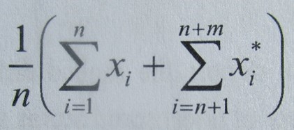
In which: x 1, 2,…n denote the runs scored by a batsman in n completed innings,  and x^* n + 1, n + 2,…n + m denote the runs scored in m not out innings.  

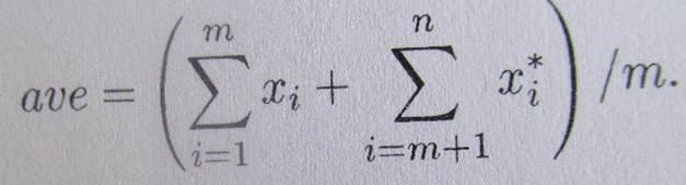
In which: x_1,  x_{2, …,} x_m  denote a batsman’s dismissal scores,  and x^*_m+1, x^*_{m+2, …}  x^*_n  denote his not out scores.

Rest assured, there is not another mathematical equation in the rest of this essay – only three understandable formula, written in words.

The Straightforward School

• These proposals address the matters at hand with much less elaborate or complicated methods (as examined in Part II).

B.  The Rarefied School

Pioneers

There are three distinct and contrasting approaches to consider. The first is a seminal contribution made by Alan C. Kimber and Alan R. Hansford in an article of ten and a half pages (plus two appendices), appearing in 1993 in the UK’s prestigious Journal of The Royal Statistical Society (JRSS). It greatly stimulated interest in the topic of how Not Out Scores should be treated in arriving at averages, and also in the associated issue of the typical distribution of batting scores (from low to high, or vice versa). Whilst the Kimber-Hansford article is, in the main, highly technical, how and why they arrive at what is advocated can be explained in non-technical terms.

Alan Kimber – seminal thinking

All except one of the 22 articles examined have been written following the appearance of the Kimber-Hansford paper. The sole exception, a study by Peter J. Danaher of the University of Waikato (New Zealand), advocated essentially the same approach. Danaher’s brief article (five and a half pages) was published four years prior to that of Kimber-Hansford in a much less known journal with a small circulation, the New Zealand Statistician. His article is rarely cited, and it is clear that Kimber-Hansford were unaware of its existence when they did their work. I shall return later on to his study and its lessons.

The background of the two authors at hand is very different:

• Alan C. Kimber: then a researcher and lecturer in statistical methods at the University of Surrey, in his mid-30s, with a specialist interest in analysis of data on materials and equipment reliability and in the modelling of survival data relating to diseases and treatments.  
• Alan R. Hansford: a Sussex county player from 1989-92, when in his early-twenties. He provided the cricket folklore, including different phases of players’ careers and the typical course of an innings, as well as most of the batting statistics.

Accordingly, I shall refer to the proposed method of deriving batting averages as that of Kimber. In effect, he followed on from where George Henry Wood left off half a century earlier. Wood was an eminent labour market statistician, trade union activist and a highly knowledgeable cricket enthusiast. His paper titled Cricket Scores and Geometric Progression was read before members of the Royal Statistical Society at its premises in the heart of London in November 1944, Wood then being in his early-seventies. It was published, along with an account of the following lively discussion, in the Society’s JRSS journal the following year (shortly before his death).

Wood was sceptical of received opinion that batsmen’s scores made in completed innings display a “geometric progression”. By this is meant they display an approximately fixed pattern, in which the number of scores achieved by a batsman typically reduce by an approximately constant ratio as the scores increase in magnitude from zero. The size of this constant tends to differ, often substantially, between one batsman and another.

Two examples of roughly geometric progressions are provided below, with the number of completed innings being given as a frequency distribution.

	G. HAYWARD	F. SIEBEL
	Number of	Number of
Runs Scored	Completed Innings	Completed Innings
0-19	53	64
20-39	36 (0.68)	34 (0.53)
40-59	24 (0.67)	19 (0.56)
60-79	18 (0.75)	9 (0.47)
80-99	11 (0.61)	4 (0.44)
100-119	8 (0.73)	2 (0.50)
120-139	6 (0.75)
140-159	4 (0.67)
Ratio of decline in number of innings:	Approx 0.7	Approx 0.5

A geometric pattern occurs if a batsman is equally likely to increase his score by a small increment (notionally, by one run) whatever score he then happens to be on. In other words, his chance of being dismissed at any time during an innings would be independent of the particular score that he has then reached.

George Henry Wood who started it all

George Wood examined the scores of three “large groups of batsmen over very many innings” (all English players at First Class level) and found materially lower survival rates in the 0-5 run range than beyond, as well as the presence of rather more innings of 80-100 and upwards, than is implied by a geometric progression. He concluded that such a progression applies “in the main to batting scores”, conforming to it over the “major part of their range”. However, he also thought it likely that the observed greater difficulty of scoring very early on in an innings, and the far greater ease of scoring when well established, are general and inherent features of the game. Various possible reasons occurred to him for the existence of these features and he was keen for these to be carefully examined.

Alan Kimber took up the reins and carefully tested for the existence of a geometric progression of batting scores at First Class level, with its key feature of approximately constant risk being faced by a batsman as his innings score progresses. The relevance of the debate as to whether or not such a progression actually holds true, and its consequence that completed scores would tend to be approximately evenly distributed from low to high, is as follows. If true, this would imply that a particular estimation procedure is valid for arriving at an estimate of the number of runs a Not Out player would have eventually scored had he batted on. The problem at hand would, in effect, be solved!

For those curious about Alan Kimber’s way of probing this issue and in knowing some of the detail of his findings, this is provided immediately below. Other readers can skip to the section following, on his approach to estimating a batsman’s “true” average.

Probing Cricketing Folklore

Kimber conducted his empirical tests for the existence of the geometric phenomenon after first noting that the received cricket wisdom – that is, widespread cricketing beliefs going back a long while that are presumed to be true – is in contrast with it. The received wisdom is that batsmen are generally most vulnerable when starting their innings, and if survive long enough – ie through a playing-in period – they become well set (though sometimes suffering from nervousness when approaching milestones). But after reaching a really big score (one hundred plus), typically doing so after some hours of batting, they tend to tire and become more error prone, and so become more liable to be dismissed.

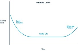
In view of this cricketing folklore, Kimber suspected that the distribution of batsmen’s scores will typically approximate to a bathtub shape (as depicted below) – drawing on a rather tenuous analogy from his familiarity with reliability engineering studies, especially rates of malfunction and physical failure over time of equipment components. Applying this analogy to batting, the “failure rate” becomes the rate of being dismissed when on different scores, and “the passage of time” becomes scoring of increasing magnitude. In the drawing below, the playing-in, well-established and fatigue phases of an innings would replace the phases noted in blue script.

In examining which of the two versions is the case, Kimber focussed, firstly,on the proportions of career scores made of zero by 9 batsmen in Test matches, by 2 batsmen in other First Class matches and by 2 batsmen in One-Day Internationals (ODIs) – al told spanning five countries. The observed proportions are found to be always higher than those implied by the geometric model: for 9 of these 13 batsmen it is 2.4 to 4.6 times higher.

Secondly, he examined the pattern of high scoring dismissals made in First Class matches by four prolific centurions (Victor Trumper, Don Bradman, Mohinder Amarnath and Dennis Amiss). The trends are clearly apparent after smoothing the innings-by-innings data plots (through applying a form of moving average).[iii] Although the data are increasingly sparse in the upper tail of the scoring distributions, dismissal rates do seem to rise somewhat in three of these four cases – doing so after 70 runs for Amarnath, after 120 runs for Trumper, and after 230 runs in the case of Bradman. But the rises in dismissal rates are small, and the profile is considered to be “quite flat at their high scores, and it seems plausible that the tail of the underlying scores distribution for a batsman is at least roughly geometric” – ie a roughly constant degree of risk is encountered.

Thirdly, Kimber applied a standard statistical test of how well the geometric progression model matches the observed distribution of scores (a “goodness of fit” test). For this, he takes a random sample of twelve sets of career scores (some for Tests, others for ODIs),[iv] and also four sets of century scores in First Class matches for Jack Hobbs, Colin Cowdrey, Glen Turner and Dennis Amiss (all with more than 100 centuries to their name). This showed strong evidence against the geometric progression hypothesis at the low scoring end. There was weaker evidence against the hypothesis in the upper tail – with some, though not pronounced, support for batsmen being more prone to dismissal at the very high scoring end.

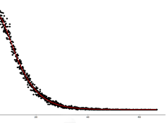
As with the surmised bathtub curve, relatively high dismissal rates occur during the initial few runs of an innings, then falling sharply to enter a long flattish phase without any persistent underlying trend; with dismissal rates seeming to rise from around the 130-150 run mark. At the low end, the graphs presented indicate that the magnitude of risk (or “hazard”) encountered starts to flatten out for Dennis Amiss at around 10 runs, and for Victor Trumper and Don Bradman at around 7 runs.

The shape of Bradman’s risk plot relating to scores of up to 50 in his First Class innings is shown below (after the data is smoothed):

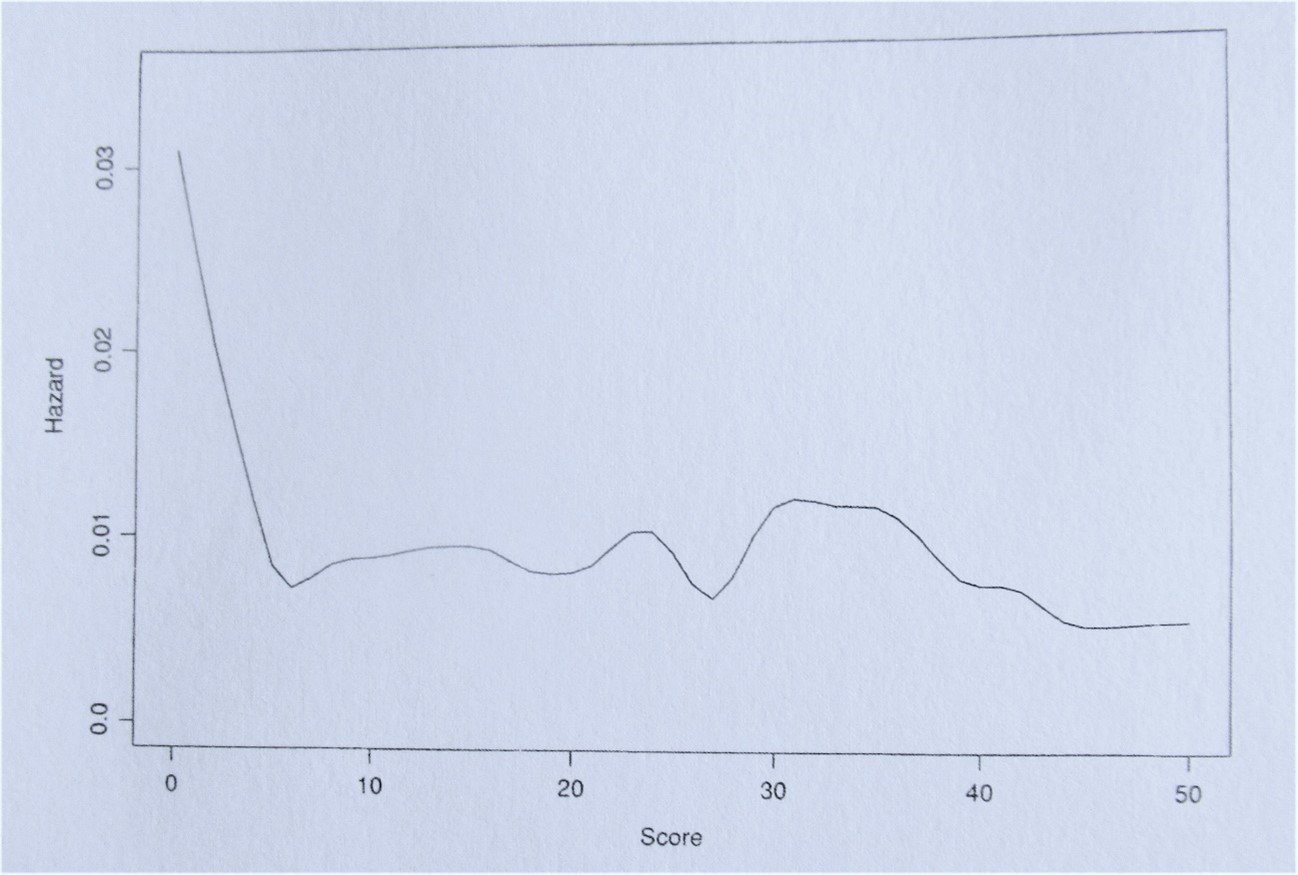
Kimber has now amply confirmed George Wood’s scepticism about notions of a geometric progression. Accordingly, if an improvement is sought on the traditionally determined batting average, a different method must be employed. The preliminary work just described constituted the bedrock for Kimber moving forward, and it takes up four and a half pages of the article.

Alan Kimber’s Approach of Determining a Batsman’s “True” Average

Kimber arrives at an estimate of a batsman’s truly representative average in two main stages:

– Applying a mechanism known as the Product Limit Estimator, which is an inherently probabilistic approach to projecting incomplete data to notionally concluded outcomes, the incomplete data here represented by a batsman’s Not Out Scores. This mechanism is his lynchpin.
– Using the resulting set of projected Not Out Scores, plus the known set of Dismissal Scores, to establish a batsman’s true average.

(i) The Product Limit Estimator Explained

This widely used tool had been devised during the 1950s by two American researchers, Edward L. Kaplan (a mathematician) and Paul Meier (a bio-statistician), their work being published in 1958 in a now famous article.[v] Significantly, the Product Limit Estimator (PLE) had its origins in the context of medical follow-up studies of a sample of patients, to show how effective a particular treatment (or type of surgery) is compared with application of a different type of treatment or taking no action. Two-thirds of Kaplan-Meier’s list of 28 references relate to papers on life expectancy, survival rates for diseases and after treatments, and follow-up health studies.

In short, these two researchers created a statistical method to determine survival rates (depicted as survival curves) for groups of patients when the available data was subject to incomplete observations of their post-treatment progress. To quote The New York Times in 2011:

“The Kaplan-Meier curve has become the standard tool used by medical researchers for determining the duration of survival in thousands of studies, ranging from cancer to AIDS to cardiovascular disease to diabetes, to name just a few.”

In monitoring the experiences of a sample of treated patients, there often arises the need to fill gaps created by those who have dropped out of a follow-up study aimed at establishing the likely timing of relapse (or death) following a treatment or surgery – such as some form of cancer treatment or kidney replacement. Such patients are lost to the study either due to their deliberate decision to no longer participate or from inadvertent loss of contact. The future course of their condition is in principle discoverable but is unknown – hidden from view, rather than being revealed – and so they become missing from the overall data set. The data collected prior to a patient dropping-out is, rather oddly, termed censored data.[vi]

Initially, the PLE’s initial role was to establish an expected (most likely) eventual outcome for drop-out patients and thereby enable the creation of a sound, comprehensive, data set for the patient sample as a whole. Those running a study would then able to make reliable statements about the likely survival prospects of future patients.

Foundation Principles

The PLE mechanism is founded on three main principles:

(a) Being lost to a follow-up study is assumed to be a random event, unconnected with the experience of other patients being monitored. For cricket, the counterpart assumption is that the occurrence of retiring Not Out is not influenced by any of that batsman’s previously completed innings.

(b) A patient having an uncompleted observation during the follow-up process should be regarded as having the same prospects of continued survival as those patients who continue to be followed-up – ie all those who have not yet relapsed (or died).

For cricket, this implies that a batsman who has to retire Not Out would have the same prospects for continued survival as when continuing to bat on having already reached that particular score and in due course completes those innings (be dismissed). In short, a batsman’s Not Out innings is treated as being represented by the experience of the array of his surviving innings at and beyond that score – which Kimber notes “is a reasonable assumption”. So he has regard had to all dismissal scores of a batsman that equal and exceed his Not Out score in question.

(c) In monitoring patients’ post-treatment progress, the survival prospects of participants who are recruited early and later on into the study are treated as being directly comparable. In other words, it is legitimate to treat later joiners in the same way as early joiners, and that the timing of joining itself is assumed not to have any influence on a patient’s survival prospects.

For cricket, this implies projecting a batsman’s Not Out score with reference to all innings played during the course of his career, or season, or the particular series of matches being examined. That is, taking account of the scores that a batsman makes both prior to, and after, a given Not Out Innings has occurred.

A fully worked example of the PLE’s use in survival analysis is provided in a readable article by Ilker Etikan and colleagues (published in 2017). They reproduce the key formula for arriving at the expected time to relapse (or death) of a drop-out patient, as given in the box below. Whilst the meaning of individual components of this formula is clear (“subjects” are patients, and “failure” is a relapse or death), the mechanics of operating the formula is a highly complicated affair. Tailor made computer software is available commercially to operate it, and so the formula can be applied by a lay person while being blissfully unaware of the mechanism churning away!

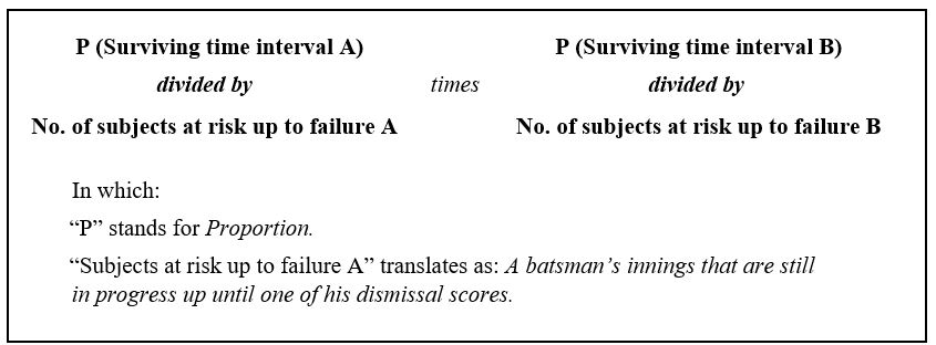
In spirit, the PLE’s approach to the gap-filling mission is to base the survival prospects of a drop-out patient on the observed survival rates (times to relapse or death) for each of all the rest of the patients who are continuing to be monitored. The crucial task is to identify the proportion of these patients who cross a given number of time intervals (such as whole months) before then relapsing (or dying), and so exit the monitoring exercise at that point.

The probability of a drop-out patient relapsing immediately upon crossing a given time interval can be estimated directly from the observations made on the rate at which of other patients relapse with the progression of time following their respective treatments. Hence, the expected time to relapse for a drop-out patient reflects the series of other patients’ relapse times and their associated probabilities. In this way, account is taken of their collective experiences. 

For those who may be curious, applying the PLE’s estimation procedure is best explained with reference to its use as part of a “survival analysis”. Other readers can skip ahead to “Kimber’s Adaptation”.

Further Detail

The following steps are involved in applying the PLE to survival analysis:

• Distinguishing patients continuing to be monitored (ie not yet relapsed or died) from those who have dropped out.
  
• Projecting the length of time that each drop-out patient can be expected to continue until they will relapse or die (ie an estimate of the most likely period), based on observed survival rates (times to relapse/death) for each of the rest of the patients. A month might, for instance, be used as the relevant interval of time.
  
• The survival rates of the drop-outs is established by:
  
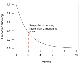
  (a) identifying the proportion of patients who survive (ie pass through or cross) successive intervals of time following their treatment without relapsing (or dying), as illustrated by the diagram below, and thereby
  
  (b) establishing the proportion of patients who pass through a certain number of time intervals before then relapsing (or dying) – and so not continuing beyond that point.

The above chart is a smoothed version of what, in practice, is a series of steps – as shown below:

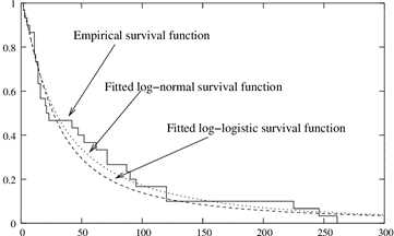
This second set of observations on the rate at which patients relapse with the progression of time following treatment, is viewed as a frequency distribution of times to relapse. The probability of a drop-out patient relapsing immediately upon crossing each time interval can be estimated directly from the relative frequencies. The higher the frequency after a given period of time, the higher the probability of the drop-out relapsing then.

(c) The likely number of time intervals to the expected relapse of a drop-out patient is given according to the mathematical notion of “expected value”, by multiplying each numbered relapse interval by its respective probability, and then summing the answers.

The plot of data with a survival curve is akin to using a life (or actuarial) table which shows, for a particular person reaching a certain age, what the probability is that they will die before their next birthday, and hence their probability of surviving any specified age. Kimber acknowledges that his own approach “is very much in the same spirit as suggested by Mr G.R. White of a batting average based on a life table” (mentioned in discussion of G.H. Wood’s paper given in November 1944).

Mr White put forward the idea of obtaining a batsman’s true average “by adding to the runs actually made an expectation of life in each of the uncompleted innings”. Although how a life table could be constructed was only tentatively broached, and Mr White himself foresaw the objection that, “One would never get the idea over to the public who follow the sporting columns of the daily papers”.

In using the PLE mechanism, the presence of information generated about a given patient surviving a certain period of time (analogously, a batsman at least reaching a certain score during an innings), and about that patient passing a particular interval of time (analogously, the batsman passing a particular score during an innings) is superfluous for arriving at a batting average. In the context of the analysis of patients, this is indeed vital information. The reason being that GPs and medical specialists actually have a much stronger interest in such information than they have in a best estimate of exactly when a particular patient can be expected to relapse or die. And the patients themselves rarely ask their GP/health adviser to give them an estimate of exactly how many more weeks/months/years they can be expected to “survive” – which is just one of the outputs from the sample patient data after the PLE has been applied.

What patients will typically want to know is, what their chances are of “surviving” (that is, not relapsing/not dying) for another, say, 3 or 5 years – or until they are, say, into their sixties or seventies. A spot estimate of their likely time to relapse (demise) will anyway, almost certainly turn out to be wrong! Even though the estimate may be the most likely of all estimates that can be made, it is most unlikely to exceed a 50% chance of being right. But for trying to predict (foresee) the future prospects for a given Not Out Innings, a spot estimate of some sort is essential!

Kimber’s Adaptation

In imaginative fashion, Kimber draws on the PLE mechanism to analyse cricket scores by making the following series of substitutions:

• the various innings played by a batsman is substituted for the set of patients under study,
  
• the progression of runs made by a batsman (ie whole numbers from zero upwards) is substituted for the progression of time from a particular starting point,
  
• having to retire Not Out (due to injury, as well as events external to the batsman himself) is put in place of a patient dropping out of being monitored, 
  
• the occurrence of a dismissal is in place of a patient’s relapse or death,
  
• a single run scored is in place of the PLE’s interval of time (a week, month, year or whatever); a batsman moves his score along in runs made, passing from a certain number of runs made to the next score. (If he hits a two or a four, these respectively stand for passing two and four intervals.)

Accordingly, in a cricket context, the expectation for a batsman as to the eventual outcome of a Not Out Innings (NOI) is based on the relative number of times he reaches different completed scores during the totality of his innings being considered. The relevant scores for projecting a NOI (those equalling/exceeding it) are depicted as a frequency distribution. The most likely potential outcome for the NOI is then based on the mathematical notion of expected value.

This value is found by assigning a probability to each of the various completed scores of relevance, multiplying their respective probabilities by their magnitudes, and then summing the resulting numbers (the “products”).

For example: a score of 5 runs that is made on three occasions should be given a probability three times as great as a score of twenty runs that is made only once. If a batsman has played a total of sixty innings, the probability of being dismissed when on 5 runs is then 0.05 (3/60).

Multiplying this answer by the score concerned (5 runs) gives its contribution to the expected value for the overall set of scores – in this example, 0.05 times 5, gives 0.25 runs.

This procedure is repeated for each of the other scores in turn, and the resulting contributions are added to arrive at the expected value.

The above procedure is equivalent to the more everyday notion of calculating a weighted average for a set of scores – ie each completed score multiplied by the number of times it has occurred, then divided by the total number of innings played.

Formally, this is also equivalent to simply adding all of a batsman’s individual completed scores and dividing the resulting sum by the total number of innings played – ie taking the Mean value (arithmetic average) of all his relevant scores.

After some trial and error, I discovered that what is a complicated and highly elaborate procedure applied, as by the PLE, can safely be reduced to the following statement:

• If a given Not Out Score is projected to its conclusion by taking the Mean value (arithmetical average) of all actually completed, and notionally completed scores that exceed and equal it, this will produce an identical result to applying the PLE mechanism.
  
• The relevant scores in this context include any other Not Out Scores which, when projected, equal/exceed the Not Out Score being considered. This iterative feature of the PLE (and hence Kimber’s) estimation procedure is logical and internally consistent. It does introduce a further complication, but this can be coped with by projecting the highest Not Out Score initially and dealing with others in descending order. (This will avoid an interminable series of re-workings.)

Proof of this exact correspondence is given by my reproducing Kimber’s estimated “true” averages for six of his batsmen using the simplified procedure described above.

This reduction is rather like a mansion such as the Palace of Versailles (a former royal residence) being recreated in all its glory though with minimal structural support. Perhaps some of the trained statisticians realise this, but are keeping it under their hats!

I believe that when writing the article, Alan Kimber was unaware that the simple method just described equated to his own in terms of results, although he would no doubt have tumbled to it if seeking to experiment. For him, it was an interesting opportunity to apply techniques he was trained in, and concepts he was highly familiar with in his professional life, to the different topic of batting in cricket. And it has turned out to be a one-off foray.

However, as discussed in Part II, use of expected values in projecting a Not Out Score to a notional conclusion is not necessarily the best guide for prediction, especially with a moderate or highly skewed set of data for a batsman’s scores.

A Special Case: If a batsman’s top score happens to be Not Out, the estimate to be made by the PLE technique is undefined; and so an assumption has to be made about the missing upper tail-end of scores. Alan Kimber bases this on evidence that, in First Class cricket at least, this end of a scoring distribution tends to display a roughly geometric progression, and so batsmen have an approximately constant risk of being dismissed as their score progresses in this region. Further, the degree of risk faced is not much different to that faced when a batsman has got an initial dozen or so runs under his belt.

Accordingly, as a general rule, a top scoring Not Out innings can reasonably be projected to an eventual outcome by adding on the average of the batsman’s scores above, say, ten runs. (This includes other Not Out Scores at their projected levels.) For those batsmen who have played at least twenty innings, the effect on their estimated “true” average will rarely be sensitive to specifying this mark a few runs either side of the nominated ten.[vii]

It is noted that a number of other researchers have subsequently devised survival curves for individual batsmen in different forms of the game. Examples are:

• Bernard Kachoyan and Marc West (2018 article) who generate survival curves for a variety of batsmen, indicating their probability of making different scores at each point in an innings – ie given the number of runs that he has already scored. They also show that these curves can be constructed from summary information that is available from a number of published cricket data bases. Results are given for the careers of six Test match batsmen.
  
• Hemanta Saikia and Dibyojyoti Bhattacharjee (2018 article) who create survival curves for batsmen in the Indian Premier League’s 2012 season. Their findings are intended for use in arranging the batting order of a team playing Twenty20 cricket, and also for making adjustments to the batting order during play so as to reflect the unfolding match situation.

(ii) Using the Resulting Set of Projected Not Out Scores

Having applied the PLE mechanism, Kimber has a single set of data to work with: the scores of all actually completed and notionally completed innings (one for each innings played). These various scores are now on an equal footing.

In this brief second stage, these two sets of scores are added to give the total runs credited to a batsman, which is then divided by his total number of innings played – so arriving at his “true” average.

Scope of Application

Kimber’s method is intended to be applicable to whole careers in Tests and in First Class matches generally, and also for innings played in a single season -16 innings being the smallest number he reports findings for, the next being 24 innings. Table 3 on page 450 of his article displays the results for nine batsmen, including some in each of these three categories.

Kimber says that in cases of a huge proportion of Not Out innings his method “is no more sensible than the conventionally estimated average”. The highest proportion of Not Out Innings for these nine batsmen is 26%. He doesn’t actually specify an upper threshold, a significant point returned to shortly.

Comparison of Kimber’s Reported Results with Traditional Averages

The resulting batting average using Kimber’s method will usually, though not always, be smaller than a batsman’s Traditional Average. The outcome depends on the batsman’s profile of scores. However, a substantial reduction will occur for a significant proportion of First Class batsmen. A typical case is a player with fairly high proportion of Not Out Innings who doesn’t make many very high scores. Provided that a batsman’s highest Completed Innings Score is greater than his highest Not Out Score, it follows that Kimber’s resulting average cannot exceed the former, which is a sound reasonableness check.

Kimber reports results for the following batsmen: Mohinder Amarnath in Tests (usually coming in at number 3), Don Bradman in Tests and in all First Class matches, David Gower in Tests (200 of his 204 innings up to time of analysis), Victor Trumper in First Class matches, and four Surrey players for the 1983 English County Championship season – Monte Lynch, in the middle order; Alec Stewart, usually at number 3; Jack Richards (wicket-keeper) in the lower middle order; and Sylvester Clarke, a tail-ender.

	Traditional Ave	Kimber’s Ave
Amarnath (113 inns, 8.8% not out)	42.50	41.40
Bradman (80 Test inns, 12.5% no)	99.94	98.98
Bradman (338 FC inns, 12.7% no)	94.76	95.14
Gower (200 inns to mid-1992, 8.0% no)	44.31	44.30
Trumper (395 inns, 5.3% no)	46.58	47.36
Lynch (39 inns, 25.6% no)	53.72	49.11
Stewart (16 inns, 18.8% no)	31.31	30.71
Richards (34 inns, 23.5% no)	27.61	27.46
Clarke (24 inns, 16.7% no)	14.25	14.15

Kimber’s adjusted average is lower in most cases, though it is a little higher for Bradman and Trumper for their First Class matches. Apart from Lynch (down 8.6%), though, the changes are quite small, with only the difference for Amarnath exceeding 2.0%.

Afterword

Rounding off their article, Kimber-Hansford put forward a proposal to extend the statistics of the number of 50s and number of 100s made by a batsman as usually provided in summary data on careers in different formats of the game. While indicating the number of times a batsman reaches or passes these two milestones, this practice stops short of informing the reader about the nature of the “past” bit.

Their proposal is to give a summary description of a batsman’s distribution of scores, and they suggest highlighting his 50^th, 75^th and 90^th centile scores (the exact choice of centiles being arbitrary). They illustrate what this implies for a selection of batsmen at First Class level, noting that the 10^th and 25^th centiles are low for the great majority of batsmen. (The 25^th centile being one-quarter up the list of a batsman’s scores, working from the smallest to largest.)

Returning to Danaher’s article, although substantial parts of his text are impossible for a lay person to follow, he illustrates the application of the Product Limit Estimator (PLE) to the innings of six players in England’s county championship, four of whom had an unusually high proportion of Not Out Innings. Deploying my simplified version of the PLE mechanism, I have replicated his finding for Martin Crowe (29 innings for Somerset in 1987 at an estimated average of 63.75). Danaher sees the main merits of using the PLE for deriving batting averages as twofold:

• producing a more sensible ranking of players’ comparative abilities, and
• rectifying anomalies with tail-enders’ averages, while still rewarding Not Out innings.

Despite the rigour and inherent appeal of the PLE approach, there is no demonstrably correct solution to completing partial data, and it is rare for the results of doing so to be tested afterwards. And in batting, there is no possibility – even in principle – of verification!

Subsequent Notables

Two very different methods are now discussed, which are those developed and applied by Lemmer and by Maini/Narayanan.

Professor Hermanus (“Hoffie”) Lemmer of the University of Johannesburg is surely the doyen of those applying statistical methods to analyse cricket data and player performance, having had at least 23 such papers published during the period 2001-17.

His Focus and Kimber’s Boundary

Lemmer tackles the problem that Alan Kimber left untouched. Recall that when a batsman’s proportion of Not Out Innings (Prop NOI) reaches a certain level, Kimber’s method of arriving at the “true” average is, in his own words, “no more sensible than the conventionally estimated average”. To anticipate what comes later in more detail, Lemmer finds that when Prop NOI reaches 40% for batsmen in the ODI format of the game, Kimber’s method becomes insufficiently reliable, and is increasingly unreliable as this proportion enters higher levels. The same problem applies to Test matches when Prop NOI becomes “much greater than around 20%”; and I assume here that this threshold can be put at approximately 23% (ie 15% higher than 20%). Kimber’s unreliability at these stages is because too little reliance is being placed on Completed Innings for projecting Not Out Scores to a notional conclusion.

It is this issue of finding a suitable method when Prop NOI is higher than a critical level to which Lemmer’s widely cited 2008a article is directed. His proposals are therefore to be regarded as filling the void that Kimber left in his wake. They are essentially a supplement to Kimber’s method, so making it more complete.

Hoffie Lemmer – Innovative Method to Fill a Void

Lemmer’s proposals take the form of two “Estimators” of the batting average. They are specified as formulae, though are ones that can readily be understood by those who don’t have a grounding in statistical matters. One of these Estimators is for general application to limited overs matches, the other for general application to Test matches and other unlimited overs matches when a batsman’s Prop NOI reaches/exceeds the thresholds just noted. For each of these formats of the game, the formula itself does not alter in any way for different batsman, even though the data needed to apply it are unique to each batsman. The data inputs are basic statistics, such as the sum of a batsman’s dismissal scores, the sum of his not out scores, the average of his not out scores and the proportion of innings in which he has remained not out. These can be easily derived from standard data on internet sites such as cricinfo and howstat.

It is significant that Kimber’s reported findings for all of his nine batsmen relate to those with Prop NOI well under Lemmer’s two markers. Specifically: Kimber’s five batsmen in unlimited overs matches have Prop NOI no greater than 13%, and his four batsmen playing for Surrey County in three day, two innings a side, matches have Prop NOI that is no greater than 26%. The latter championship matches are more akin to limited overs matches than to Tests in view of their time-scale, especially as bad weather has often reduced playing time by at least half a day. (In all, 13 of Surrey’s 24 championship matches that season were drawn. Three of these draws ended with no more than one and a half of the potential four innings being played, and another three draws ended with no more two and a half innings being played.)

At this juncture, it is necessary to probe a potential disconnect between the respective statements of Kimber and Lemmer. When mentioning the boundary for the proportion of Not Out Innings applying to his own method, Kimber uses the term “huge”, while Lemmer uses the term “large” (proportion) as the focus of his Estimators. To tell whether Lemmer’s markers of 40% and 23% are in conflict with Kimber’s stated limit, “huge” has to be interpreted as Kimber didn’t comment further. There are two ways he may have looked at it.

The first relates to an abstract scale, ranging from, say, zero up to a maximum of 100%, with all levels being equally likely to be reached. A proportion of 90% or 95% and upwards could then be taken as representing his (and most people’s) idea of what represents huge. But it seems more likely that Kimber thought of huge within the context of batting statistics and his appreciation of what is a rare or unusual proportion of Not Out Innings – the following observations being pertinent:

ODIs and their ilk

• Since ODI matches began in 1971 through to mid-December 2021, there are 113 England players with a minimum of 14 innings: of these, eighteen reach or exceed the threshold of 40% NOI – that is 16%. All except three of the eighteen are tail-enders. (Only three of the players, all being tail-enders, have Prop NOI of 50% or more.)
  
• For all countries since 1971 through to mid-December 2021, there have been 99 players with a minimum of 20 innings and an official average of at least 38.0 and so they are specialist batsmen or genuine all-rounders. Of these, just 1 player has Prop NOI exceeding 40% (Imad Wasim of Pakistan, at 42.5% for 40 innings – the next highest is 36.5%, applying to two players).
  
• Taking the three day matches of the 1983 English County Championship, which Kimber drew on: of the 205 players with a minimum of 14 innings, only 6 of them – just 3% – have Prop NOI reaching/exceeding 40%. These are all tail-enders.

This evidence suggests that Lemmer’s 40% marker is rarely met in the limited overs format, except in the case of tail-enders and even for them this is an unusual occurrence.

Test matches and their ilk

• In the case of England players since Tests were initiated through to mid-December 2021: of the 229 players with a minimum of 20 innings, there are 32 – ie 14% – with Prop NOI reaching or exceeding 23%. All of them are tail-enders. (A further 6 players have Prop NOI of 20-22%, all except two being tail-enders.)
  
• Taking the four day matches of the 2018 English County Championship, Division 1: of the 64 players with a minimum of 14 innings, only 5 – ie 8% – have Prop NOI reaching/exceeding 23%.All these are tail-enders. A further three players have Prop NOI of 20-22%, and again they are tail-enders.

This suggests that meeting Lemmer’s 23% marker is extremely rare for specialist batsmen and all-rounders, and even for tail-enders it is unusual.

In conclusion, Kimber and Lemmer are not fundamentally in conflict over this boundary issue. Defusing it has been worth the effort and length of exposition involved as an adjudication would otherwise have been needed!

Roles that Lemmer’s Estimators Can Play

For those wanting to apply Lemmer’s Estimators of a “true” average to batsmen’s whole careers, these clearly have a very limited role to play other than for tail-enders. But for a short series of matches, his contribution ceases to be of a niche nature and has a wide application. Examples are:

• The ODI and Twenty20 World Cup competitions – respectively giving each batsman up to 11 innings and 7 innings.
  
• A single series of ODI or Test matches, the latter typically having potential for 6-10 innings.
  
• The Royal London One-Day Cup competition: for season 2021, producing 11 innings in the case of one batsman, the next highest being 9 innings.
  
• A season in the Indian Premier League which provides for up to 14 innings, plus the play-off matches.

In one particular short series, the inaugural Twenty20 World Cup competition, Lemmer applied his recommended Estimator to a number of innings played as low as three (2008b article).

In deriving his recommended Estimators, Lemmer employs standard statistical techniques – except for one ingenious move that I shall draw attention to in due course. What is of relevance here is the underlying logic which I try to lay bare in the following sections. This is needed if a lay person is to have confidence in the results to be obtained from their application.

Why Kimber’s Method Produces Unstable Results, at Some Stage

The first and crucial thing to uncover is why it should be that Kimber’s method of determining a “true” batting average becomes unreliable when Prop NOI reaches a certain level, having worked satisfactorily before then. (Recall that his method centres on projecting Not Out Scores to a notional completion by taking the mathematically expected value of all the scores that exceed or equal it.) This can be explained, at an intuitive level, by noting that the number of relevant scores on which to base the projections of Not Out Scores (NOSs) becomes fewer and fewer as a batsman’s Prop NOI increases.

At some point, further small reductions in the number of relevant scores have a large and erratic effect on the resulting projection, leading to the estimated “true” average becoming unstable. This reflects the tendency for the available scores on which to project NOSs then becoming sparse and patchy.

The relatively large effect of a small change in number of Dismissal or Not Out innings is seen in the case of Steven Finn’s Test match career of 47 innings and Prop NOI of 47%. Deleting two Dismissal Innings of scores of 17 and 19 runs (in a starting total of 25 Dismissal Innings and 213 runs) leads to an increase of 8% in his total projected Not out Scores. And deleting one Not Out Innings, of a score of 16 (in a starting total of 22 Not Out Innings) produces a 5% reduction to his estimated “true” average.

Principal Features of Lemmer’s Method

Instead of using the raw data on scores to drive the analysis, as Kimber did, Lemmer works with a statistical curve to represent the distribution of a batsman’s scores (from high to low). In summary: working with carefully selected samples of ODI batsmen and Test batsmen, he ultimately combines the scoring data for the most suitable nine batsmen for each of these formats, having first projected all of the Not Out Scores to a notional conclusion. The set of aggregated data on ODI scores – and the aggregate data on Test match scores – can then be thought of as relating to a single “composite” batsman in each case.

Lemmer fits a curve to the aggregate data on ODI scores, finding the shape of curve that gives the closet match to the data set. Given the exact shape of the curve, its Mean value (ie the arithmetic average) can be found using a standard rule. This value represents the “true” batting average for his collection of nine ODI batsmen. The final step is to determine a precise formula that gives the same answer as that Mean value, or a very close approximation to it. This is his “Estimator” for general use when an ODI batsman’s Prop NOI reaches/exceeds the 40% threshold. The same procedure is followed with the aggregate data on scores for the nine Test match batsmen.

The Estimator for each format of the game can then be applied to a given batsman without reference to any fitted curve and rely, as mentioned earlier, on a few readily available performance statistics.

For those wishing to know something of the supporting detail, the main steps are elaborated on below. Otherwise, the reader can skip ahead to the sub-heading “Specific Form of the Recommended Estimators”, after which the effect of applying the Estimators is examined and compared with the results of using Kimber’s method.

The Samples of Batsmen – ODIs and Test Matches

Lemmer works with random samples of specialist and all-rounder batsmen, drawn from the entire pool of then current players (as at mid-August 2005), spanning all participating countries. All are well established players and nearly all have moderate to strong official averages (the lowest being in the twenties).

For ODI matches, he works initially with 22 batsmen who, with just two exceptions, have played at least 100 innings. He needs a high number of scores for each batsman in order to make his statistical analysis sufficiently reliable for practical application. In particular, this enables a good fit to be achieved when superimposing a standard type of statistical curve on the scores made by a given player. The five players with the highest Prop NOI are in the 30-37% range; the next four players spanning 20-29%, with most of the other 13 players spanning 8-18%.

For Test matches, Lemmer works initially with the scores for 20 experienced batsmen, each with at least 100 innings (ranging from 103 to 179). Overall, their Prop NOI are much lower than for ODIs – the highest six being in the range of 13-19%., reducing down to only 5%. 

In projecting each of a batsman’s NOS to notional conclusion – referred to as an augmented or complete score – Lemmer has regard to scores made throughout the batsman’s career. He converts each NOI into a complete score by taking the mathematically expected value of those scores.[viii] Each relevant score is assigned an equal probability of occurring. (Accordingly, if there are three innings played each of 25 runs, the score of 25 is given three times the probability of a score of 35 runs made in only one innings.) This amount to exactly the same thing as taking the Mean value of all the separate individual scores that equal or exceed the NOI in question.

In doing this, account is taken of other Not Out Scores at their projected values. It is noted that Lemmer’s procedure for projection produces an identical result to Kimber’s method of doing so using the PLE mechanism (as described earlier).

Each Not Out score is replaced by the “augmented” score and included alongside all actually completed scores to give a single set of scores for each batsman, as a basis for Lemmer’s curve fitting exercise.

Fitting Statistical Curves to Batsmen’s Scores

In summary, Lemmer superimposes a statistical curve on the array of a batsman’s ODI scores (arranged from high to low) and, separately, does this also for the array of a batsman’s Test match scores. Numerous possible shapes of curve are tried out and from these the one that most closely matches the scores data is identified.

Fitting such a curve to batting scores acts as a trend line through the distribution. In effect, it provides a smoothed version of the raw data on individual scores. So the actual distribution of scores made will depart somewhat from the fitted curve – deviating upwards from the curve along some parts, downwards along some other parts. Also, while the fitted curve will consist of a continuous series of data points, with the raw data series there will be some discontinuities along the progression of sores made (from high to low). These two types of disparity won’t be of material consequence so long as the fit to the data is close.

Achieving a very close matching to the raw data on a batsman’s scores, so that the curve is a very good representation, is essential for Lemmer’s aim of arriving at reliable Estimators of the batting average – as he himself stresses.

To elaborate: statistical curves of different types are fitted to the scores of each batsman and are then assessed for matching. These are chiefly curves of the so-called Gamma and Weibull families. Examples of the Gamma family are shown below, being widely used in various fields of science to model data on variables that have skewed distributions – as typically applies to batting scores.

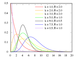
A striking feature of both the Gamma and Weibull families is the very different shapes these distributions can take. Their versatility means there is strong potential to give a good approximation to typical patterns of batting scores. The two left-to-right downward sloping examples of the graph are of potential relevance.

The best shape of curve for each batsman is established by applying a standard statistical technique known as “maximum likelihood estimation”. The exact shape it takes depends on the value specified for its two parameters.

Example of a fitted Gamma type curve and the raw data on scores

The comparative performance of the best Gamma curve and the best Weibull curve for each batsman was assessed by establishing the maximum distance between the scores made and the fitted curve – smallest distance being best. Lemmer finds that a Gamma type of curve is, in overall terms, best for both his ODI and Test match batsmen. The exact shape it takes varies from one batsman to another, reflecting the variation in their scoring profiles.

The resulting “true” averages for the two samples of batsmen were derived directly from a given batsman’s fitted curve by dividing the value for one of its two parameters by the value for the other. Lemmer finds that the estimated batting averages have a very close correspondence with those obtained by an alternative method that makes no use of statistical curves, providing that the proportion of Not Out Innings for the batsmen concerned is well below his critical threshold levels (40% for ODIs and around 23% for Test matches). The alternative is simply to take a batsman’s set of projected Not Out Scores, add these to his Dismissal Scores and then divide through by the total number of innings played. This correspondence justified a high confidence being placed in the curve-fitting approach going forward when high proportions of Not Out Innings are considered.

A Dilemma and an Ingenious Solution

However, Lemmer finds himself on the horns of a dilemma because the requirement for having a large number of innings played by the various batsmen comprising his samples was incompatible with wanting to find a suitable Estimator for Prop NOI of 40% (and upwards) for ODIs and of around 23% (and upwards) for Test matches. As his two samples are comprised of whole careers of specialist batsmen and genuine all-rounders, it was inevitable that their Prop NOI would fall short of these markers. For those batsmen with the very best curve fits (9 of the 22 for ODIs, and 9 of the 20 for Test matches), the highest Prop NOI is only 24% in the case of ODIs and only 17% for Test matches. And it is these batsmen who are retained for the rest of his study, precisely because of their very good curve fits. (Each of them had played at least 160 ODI innings or at least 130 Test match innings.)

Giving up either the composition of his chosen 9 ODI and 9 Test match batsmen or his associated thresholds was not only highly undesirable, it would have been self-defeating! And Lemmer couldn’t use data on a short series of matches to produce batsmen with the desired Prop NOI because they wouldn’t have played enough innings to achieve very good curve-fitting and reliable results![ix]

Lemmer resolves this dilemma in an ingenious way. For each of the chosen nine ODI batsmen and nine Test match batsmen, he transforms a sufficient number of their Dismissal Scores into equivalent supposed Not Out Scores, so as to attain the desired 40% and 23% Prop NOI. He does this “down-scaling” for a given batsman by applying some of his own ratios of actual Not Out Scores to their projected completed scores (one particular ratio, or relationship, applying to each NOS). Both the particular Dismissal Scores to be transformed, and the ratios to be applied to them, are selected in a random manner.

For example: in the case of Abdul Razzaq (one of the nine chosen ODI batsmen), 67 Not Outs scores are required but he has only 41 actual Not Out scores, and so 26 of his 127 Dismissal Scores have to be down-scaled. Each transformed score is subsequently scaled back up using the inverse of the down-scaling ratio, thereby being returned to its original value. All the chosen batsman will now have a suitable, revised, set of scores that Lemmer can work with. Each of them will get a revised curve fitted to their scores as their original Not Out Scores have been projected differently, there being fewer relevant Completed Innings Scores on which to base the projections.

Although this down-scaling exercise does seem to have logic on its side, a lay person can be forgiven for thinking that we have now stepped into Alice in Wonderland territory – Lewis Carroll’s tale, published in 1865, which still shines as part of the literary nonsense genre.[x]

Finding Reliable Estimators of the Batting Average – for ODI & Test match scores

Another key move was now made by Lemmer. This was to pool the set of data for the nine chosen ODI batsmen and likewise for the nine chosen Test match batsmen. In each case, a best fit curve was applied to the scores of the nine batsmen collectively – ie to their aggregate data – so that a generally applicable Estimator could be identified. Without such pooling, different Estimators would have emerged for the individual batsmen and no concrete recommendations for arriving at “true” averages could have been formulated. (Pooling also, incidentally, countered the tendency for the scores made at the high end of the batsmen’s distributions to be thinly spread or patchy.)

For each of the two formats, numerous alternative possible Estimators were formulated and evaluated according how well they reflected the shape of the batsmen’s collective curve, this being done using a conventional statistical test (the root mean square error criterion).

Lemmer’s three best Estimators for each format, which all performed “reliably”, were then compared with Kimber’s Estimator and the Traditional Average formula. Lemmer’s three are shown to decisively out-perform the other two at the 40% and 23% NOI markers, the more so with still higher proportions of Not Out Innings. His own very best Estimator for each format performed “very reliably”.

Specific Form of Lemmer’s Recommended Estimators

For ODIs and other limited overs matches

The Estimator version referred to as “e₆” was found to be the most suitable for these matches, as well as being easy for non-specialists to calculate. It takes the form specified below.

Sum of Dismissal Scores plus (f₆ times the Sum of Not Out Scores),

 divided by Number of Innings played.

     in which  f₆ = 2.2 – (0.01 times the average of Not Out scores)

The symbol f in the formula is the factor by which a Not Out Score is scaled up to obtain a notionally completed score. For instance, if the average of a batsman’s Not Out Scores is 35,  f would have a value of 1.85 (2.2 minus (0.01 times 35)) and his Not Out Scores, totalled up, would be multiplied by that number and then added to the total of his Dismissal Scores. The resulting answer is then divided by the total number of innings played to give his “true” average.

For Tests and other unlimited overs matches

The most suitable Estimator for these matches was found to be “e₈”, which is given as:

Sum of Dismissal Scores plus (f₈ times the Sum of Not Out Scores),

divided by Number of Innings Played.

    in which  f₈ = 2.2 minus (0.01 times the average of Not Out Scores) plus

    (0.15 times the proportion of Not Out Scores).

    The proportion of Not Out Scores is expressed as 0.15 (for 15%), 0.35 (for 35%), etc.

Note that the relative emphasis placed on the individual components of the two formulae varies, and so their respective degree of influence on the resulting average differs.

Most notable in the category of unlimited overs matches, besides Tests, are Australia’s inter-state competition, West Indies regional competition (formerly the Shell Shield), South Africa’s inter-provincial competition and, from 1993 onwards, the English County Championship – all these matches being played over four days and hence of similar duration to Test matches (three to five days).

Impacts on Batting Averages Compared with Kimber’s Method

Limited Overs matches

In their review paper of 2011, Paul van Staden and colleagues (University of Pretoria) examine what Lemmer’s “e₆” formula and Kimber’s method estimate for a group of nine players who participated in the limited overs format of the 2010 Indian Premier League. These batsmen each had between 7 and 16 innings, including at least one Not Out innings.

Three of these players had their proportion of Not Out Innings (Prop NOI) above 40% (Lemmer’s marker): Mithin Manhas at 50%, and Kevin Pietersen and Adam Voges at 43%. Both Lemmer’s and Kimber’s method gave results lower than the Traditional Average.[xi]

Lemmer’s resulting averages are higher than those of Kimber for all nine players, the following points being of interest:

• The difference between the two sets of averages tends to get larger (in percentage and absolute terms) as Prop NOI increases.
  
• For the four cases of Prop NOI between 23% and 31%, Lemmer’s resulting averages work out substantially higher than for Kimber (one-sixth higher).
  
• For two of the three batsmen with Prop NOI of at least 40%, the differences are large: Lemmer’s average being 32% and 39% higher than for Kimber. In the other case, that of Kevin Pietersen, the difference is small (Lemmer’s being 6% higher than Kimber’s). This is a reflection of the fact that Pietersen’s top score was a Not Out and his two other Not Outs were his third and fourth highest scores in a generally low scoring series of seven innings.

Three day, two innings a side matches (akin to ODIs); and Test matches

For the seven batsmen that Kimber reported his findings, their respective Prop NOI are well below Lemmer’s thresholds, and so comparisons of batting averages using their two methods are of limited interest. Suffice to say that the two sets of averages derived for six of these seven batsmen are quite close, all being within one run per innings and three of them being within 0.4 run per innings.

This closeness reflects the fact that their respective ratios of Not Out Scores to projected completion for these batsmen are quite similar. Lemmer’s multiplier ranges from 1.77 to 2.08 for the four batsmen in ODI type matches, and from 1.39 to 1.60 for the three Test match batsmen; while Kimber’s multipliers for these two groups range, respectively, from 1.75 to 1.92 and from 1.49 to 1.82.

The general nearness to a multiplier of 2.0 is noteworthy and reassuring. In his 2008a article, Lemmer contends that under the following assumption – that the external factors which could curtail a batsman’s innings without him being dismissed are random and independent of his potentially completed score – then, on average, he could be expected to have doubled his undefeated score.

Although Lemmer doesn’t supply the associated reasoning, an expected general multiplier of around 2.0 may be explained in this way. Given a very large number of Not Out Innings and also of Completed Innings, the distribution of a batsman’s (stranded) Not Out Scores would likely range from an approximation to the average of his Completed Innings Scores (ie being fully fulfilled) through to his lowest Completed Innings Score which is usually zero (being wholly unfulfilled). With very numerous innings played, a fairly even distribution of Not Out scores could be expected between these two values, with an overall Mean value at around half the average of the batsman’s Completed Innings Scores. Hence, Not Outs would, in aggregate, be doubled to reach total completion scores.[xii]

Turning now to Sanchit Maini and Sumit Narayanan, two professional actuaries who diverted from their usual work to produce a novel method to correct for the defects they perceived with the traditional batting average. Their proposed method is explained in a two page piece published in 2007.

Having aired their distrust of the Traditional Average as a reliable measure of central tendency – ie as being representative of a batsmen’s overall distribution of scores – these authors propose a method of arriving at batting averages that draws on an analogy with the concept of exposure to risk, as applied in the world of insurance. This method does have its attractions and is often cited in the literature, even getting exposure in The Economist magazine.

In essence, Not Out Innings (NOIs) are converted into a number of completed innings equivalents by identifying the number of deliveries faced and comparing that number with the number of deliveries faced per completed innings when taken over the batsman’s whole career. For convenience, I refer to the latter as the batsman’s “career grand average”. (The authors don’t actually use the term completed innings. Yet if all innings is applied instead, their solution would often make little sense. So I assume the former does apply.)

I am satisfied with the whole career basis (either finished or still in progress), rather than number of innings played up to the occurrence of a NOI in question, for reasons given in Part II where this issue crops up acutely.

A batsman’s career grand average is denoted by 1.0. Each NOI has some degree of associated exposure to risk, and is given a proportional fraction of 1.0 if the number of deliveries faced is less than his career grand average. These pro rata fractions are added together to give the batsman’s number of equivalent completed innings.

If the number of deliveries faced in a NOI is equal to, or greater, than his career grand average, it is accorded a full 1.0 – equating to one completed innings which then contributes to the denominator, ie his number of actual and equivalent completed innings. Total runs scored are then divided by that number of innings to arrive at the average that represents his demonstrated capability.

Accordingly, the degree of risk exposure for a NOI is capped at the batsman’s career grand average for the number of deliveries faced in completed innings. To assign a value of greater than 1.0 if he survives greater risk exposure than his career grand average would be perverse, as it would penalise him for an above normal stint of survival. I am uneasy about the fact that a batsman who survives beyond his career grand average and remains Not Out is, nevertheless, treated as having played a “full” innings for calculating his representative average.[xiii]

Perhaps a way around this problem would be to identify the average number of deliveries received in those completed innings that equal or exceed the batsman’s career grand average, and then state the NOI in question as a fraction of that number. If there are multiple innings of this nature, the fractions would be added.

The Maini/Narayanan method has the merit of rewarding relatively fast scoring in playing a Not Out Innings, though it penalises a batsman for slow scoring which may have been justified, as in trying to stave off defeat or facing high class bowling.

Unfortunately, despite its attractions, the proposed approach cannot be implemented for many former batsmen as the number of deliveries faced has often not been recorded, or at least not preserved, for Test matches (let alone other First Class matches) – such as the West Indies versus India series of 1952/53, England versus West Indies in 1957, India versus England in 1961/62 and Sri Lanka versus Pakistan in 1986.

NOTES

---

[i] With the traditional calculation of a batting average, the total of the Not Out Scores (NOSs) are spread across all of the Completed Innings Scores – eg a NOS of 8 runs may be spread over 4 completed innings totalling 30 runs, so adding a premium of a further 2 runs to a Completed Innings Average of 7.5 to give 9.5. This is equivalent to projecting that NOS to a Dismissal Score of 17.5 runs, giving a total of 47.5 runs for what are now 5 “completed” innings (so maintaining the stated overall average of 9.5). When a Not out Score is projected to a completion, that in effect increases the number of completed innings by one, and so the premium has to be applied to the projected NOS as well.

[ii] This rarely happens in practice; when it does it is usually for a batsman who has played up to around half a dozen innings.

[iii] The form applied is termed exponential smoothing as exponentially decreasing weights are used as one moves forward across the distribution of plotted completed scores from low to high (or high to low). This technique is often used for analysis of time-series data.

[iv] The 12 sets of scores were for Allan Border, Ian Botham, John Emburey, Gordon Greenidge, Kim Hughes, Viv Richards and Jeff Thomson in Tests; and for David Gower, Desmond Haynes, Imran Khan, Javed Miandad and Kris Srikkanth in ODIs.

[v] This article was a lengthy time in the making, when Kaplan was at Bell Telephone Laboratories in New Jersey and Meier was at John Hopkins University in Baltimore. Independently, they did related research beginning in 1952/53 and submitted separate manuscripts to the Journal whose editor persuaded them to produce a joint (merged) version. Correspondence spanning a number of years was required to reconcile somewhat different approaches to addressing the problem.

[vi] The analogy is presumably with censorship in the arts and literature, much like some lines in a stage play being suppressed by a government official and so are missing from the live performance.

[vii] Kimber’s modelling is equivalent to converting a top score Not Out Innings to an estimated completed score by adding on the overall average of all of a batsman’s scores. My recommendation is a refinement that nullifies the high risk typically faced early on in an innings.

[viii] This was deciphered for me by Hoffie Lemmer, making reference to the formidable looking equations given in his 2001 article (Section2, page 46), from which was derived the summary equation on page 69 of his 2008a article.

[ix] If Lemmer had selected tail-enders, most of them may have had NOIs of 40% plus, but he would then be unable to test the reliability of using curve fitting against the alternative method just noted.

[x] The down-scaling undertaken seems to be no less outlandish than, for instance, a university that has too few undergraduate students to qualify for an uplift in its government grant, employing a time machine to convert many of its post-graduates into their former pre-graduate selves. I’ll leave the reader to imagine parallel examples within the context of Carroll’s fantasy tale.

[xi] In their review article of 2016, P.K. Gaur and D. Bhattacharjee (Assam University, India) examine the estimated batting averages that Lemmer’s “e6” version (and some other proposals) produces for a group of 20 players who participated in the 2015 ODI World Cup (played in Australia and New Zealand). However, for none of these players does the proportion of Not Out innings reach Lemmer’s marker of 40%  – the closest being M.S. Dhoni at 30%, and A.B. de Villiers and K. Sangakkara at 29%.

[xii] There is a supportive analogy here with application of the rule-of-a-half applied by economists in valuing the time saved by those making additional vehicle trips following a highway improvement scheme. In the absence of empirical evidence, the extra trips so generated are assumed, on average, to produce a benefit approximating to half of the time savings accruing to the base-load of trips (ie those made prior to the improvement in travel conditions.) At maximum, an induced traveller can be expected to benefit at the full extent experienced by the base-load travellers, and at minimum by a minimal amount. The reasoning is that some additional trips would be induced even by a very small reduction in travel time whilst, at the other extreme, some trips would only just be induced by the full reduction made to travel time; and it is assumed there is a continuous and even distribution of induced trips between these two limits.

[xiii] Although a batsman is partly rewarded for his longer survival through any additional runs he makes, this is beside the point (and, in such a case, he might actually make fewer runs than when playing innings in which he has faced less than his career grand average).

REFERENCES

P. Barton: Do Tail-Enders’ Batting Averages Benefit From Not-Outs? The Cricket Statistician Journal, Autumn 2015 (pp 18-20).

P.J. Danaher: Estimating a Cricketer’s Batting Average Using the Product Limit Estimator.
The New Zealand Statistician. June 1989 (pp 2-5).

K. Date: The Calculus of the Batting Average. Cricinfo website, 29 May 2014 (6 pages).

I. Etikan, S. Abubakar and R. Alkassim: The Kaplan-Meier Estimate in Survival Analysis.
Biometrics & Biostatistics International Journal, February 2017 (pp 55-59).

H. Ganjoo: How to Account for Not-Outs More Accurately When Assessing Batsmen.
Cricinfo website, 27 May 2018.

P.K. Gaur and D. Bhattacharjee: On Finding the Most Compatible Batting Average.
Journal of Applied Quantitative Methods, September 2016 (pp 50-60).

B. Kachoyan and M. West: Deriving an Exact Batting Survival Function in Cricket.
14^th Australasian Conference on Mathematics in Sport, July 2018.

E.L. Kaplan and P. Meier: Nonparametric Estimation from Incomplete Observations.
Journal of the American Statistical Association, 1958 (pp 457-81).

A.C. Kimber and A.R. Hansford: A Statistical Analysis of Batting in Cricket.
Journal of the Royal Statistical Society, 1993 (pp 443-55).

H.H. Lemmer: Estimation of the Batting Ability of South African International One-Day Cricket Players. South African Journal of Science and Technology, Issue Number 2, 2001 (pp 45-48).

H.H. Lemmer (2008a): General Measures of Batting Performance in a Short Series of Cricket Matches. South African Statistical Journal, Issue No. 1, 2008 (pp 65-87).

H.H. Lemmer (2008b): An Analysis of Players’ Performances in the First Cricket Twenty20 World Cup Series. South African Journal for Research in Sport, Physical Education & Recreation. Issue No. 2, 2008 (pp 71-77).

S. Maini and S. Narayanan: The Flaw in Batting Averages. The Actuary (UK journal),
May 2007 (pp 30-31).

H. Saikia and D. Bhattacharjee: Survival Ability of Indian and Overseas Batsmen on the Cricket Pitch in Indian Premier League. MOJ Sports Medicine, Issue 4, 2018 (pp 113-16).

P.J. van Staden, A.T. Meiring, J.A. Steyn and I.N. Fabris-Rotelli: Meaningful Batting Averages in Cricket. South African Journal for Research in Sport, Physical Education & Recreation. January 2011 (pp 75-82).

G.H. Wood: Cricket Scores and Geometric Progression. Journal of the Royal Statistical Society,
1945 (pp 12-22).