Making All-Time Test Batting Averages Fully Comparable
Peter Kettle |
Making All-Time Test Batting Averages Fully Comparable
When scanning a collection of men’s Test career batting averages such as this:
Don Bradman 99.9
Graeme Pollock 60.9
Len Hutton 56.6
Viv Richards 50.2
Virat Kohli 48.7
Hanif Mohammad 43.9
Michael Slater 42.8
Bobby Abel 37.2
many cricket enthusiasts would be tempted to treat the differences as indicative of relative ability, while realising that they are not fully comparable owing to the different periods in which they played and their different scoring contexts. This would be similar to comparing the absolute level of wages paid for certain occupations from one generation to another without taking account of the rate of increase, or decrease, in consumer prices and its impact on purchasing power – so falling prey to “money illusion”.
The main aim of this article, reflecting these comments, is:
– to enable valid comparisons to be made of prominent batsmen’s career averages across generations since the start of Test matches in the late-1870s, and to show what this implies for their relative standing; and
– as a secondary concern, to determine if Don Bradman really can be regarded as an anomaly, a lone star detached from the rest of the field – in statistical terms, a classic “outlier”.
In terms of scope, I have limited this in recent times to the ten main Test playing countries, being those competing for the ICC’s Test World Championship plus Zimbabwe which gained Test status in 1992 (hence ruling out the likes of Ireland and Afghanistan). The content updates the findings of my initial attempt in 2018 and, in doing so, makes a number of significant improvements to the methodology then applied.[i]
There are, of course, quite a number of interesting ways in which batting performance for different careers has been evaluated – incorporating factors such as strike rate, consistency of scoring, proportion of fifties or centuries made and contributions to team wins. Yet the traditional “runs scored per completed innings” retains its interest as a readily accessible single, and frequently quoted, statistic of demonstrated ability. Hopefully, the findings of this analysis will add value when the “official” (or raw) averages of certain players are compared and discussed by commentators and writers, and by cricket followers at grounds, clubs and at home.
The Backdrop: Changes to the Norm and Spread of Batting Averages
The “central level” of the mass of Test career batting averages, and the extent of their spread around that norm, have altered materially from one era to another, as outlined below. As will be seen, both features need to be allowed for in putting averages of past eras on an equal footing with those of the present day.
Scoring levels (for those with a minimum of twenty innings) have been subject to both sustained increases and decreases over a number of decades as well as to some shorter-term fluctuations. Scoring was particularly low during the initial decades – with an overall average of 19.0 for 1877-89, primarily owing to rudimentary pitches – rising to 26 for 1900-14 and continuing on to reach 33 for the twenty year inter-war period. The norm fell back during the 1950s and ’60s to around 28, with fluctuations occurring since then, to stand at 29.9 for the 1990s and at 27.2 for the new millennium.
These alterations to scoring levels over time reflect, in part, changes occurring to the playing context – ie the terms on which the contest between bat and ball takes place. Some examples: changes favouring batsmen have included major improvements to the condition of pitches from the late-19th century through to the 1920s and the introduction of weather protective covers in the 1960s and ’70s; while changes to playing regulations (chiefly, the often altered LBW rule, allowed number of leg side fielders and number of bouncers per over) have sometimes altered the balance in favour of the bowlers, though more usually favouring batsmen. Among other changes, there have been innovations in protective equipment for batsmen (eg helmets).
Also at work has been the relative speed of development of batting and bowling skills, including a broader repertoire of shots and of pace and spin deliveries. In some periods, advances in batting have lagged behind those of the bowlers, whilst in other periods it has been proceeding more quickly than the bowling (such as the inter-war period). This relativityof the stage of evolution reached by these roles at any given period has therefore also affected the balance between bat and ball and resulting scoring outcomes.
In parallel, the amount of variation in the performance of batsmen alone – manifest as the extent of spread around the central level of scoring – has been steadily and systematically reducing over the past one hundred years. As Stephen Jay Gould of Harvard University has convincingly argued for baseball, and also for professional sport in general, a contraction in performance variation is to be expected between successive generations. This is due to the operation of two main factors: [ii]
- A general improvement, and greater uniformity, occurring with the maturing of a sport – stemming from a more widespread dissemination of best practices and advances in techniques, higher standards of fitness, more individually directed coaching and suchlike. (In baseball, the improvements have applied to batters, pitchers and fielder positions alike.)
- A ceiling ultimately coming into effect as the elite performers approach the limits of human attainment.
In cricket, following the resumption of first-class matches after WW1, the reduced spread of averages has been due to these trends – characterised as the gradual development of “professionalism”.
The Task of “Standardising” Batting Averages
One cannot simply “update” a past player’s average by an index that reflects the subsequent change in the overall level of batting averages from one period to another. This is mainly because the rate of change is far from uniform across the spectrum of averages from low to high and so it isn’t possible to “track” the notional change to a particular batsman’s average through time.
Producing a set of fully comparable averages requires a way of taking account of – in effect, neutralising – the changes occurring over time, subsequent to a player’s career, to both the playing context and skill relativities of the batsmen and bowlers. It also requires a way of reflecting subsequent changes to the spread on averages.
Approach Adopted
Although the task of allowing for such changes is, on first sight, a formidable one, it can be greatly simplified by a suitable specification of eras and applying “dominance ratings”, as done here. The overall passage of time is divided into individual eras for which scoring levels and their spread have been relatively stable, so that the different averages attained within a given era are roughly comparable (though, in contrast, not across eras).
Standardising the “official” averages has then involved three main tasks, undertaken sequentially:
(i) Discarding the runs a batsman makes which are of no material value to the team – termed “dead runs”.
(ii) Establishing the extent of each batsmen’s dominance in his own playing period, and converting these ratings into equivalent averages within the scoring context of the Present Era.
(iii) Adjusting the resulting set of averages to allow for the general advance over time in batting expertise.
This model, capturing the influence of just three factors, is straightforward to apply. On considering the method and findings obtained, the reader may wish to introduce additional factors they consider would then produce a better reflection of the batsmen’s relative abilities at the crease. These “extensions” could be thought of as representing refinements to the basic scheme applied here – as discussed, with some potential examples, at the end of this piece.
A total of 173 batsmen were selected for the exercise, comprising those leading the official averages in each of eight defined eras through to mid-July 2023:[iii]
1877-89 1890-1914 1920-39 1946-66 1967-79 1980s 1990s 2000-23
6 10 13 31 17 17 18 61
3.5% 5.2% 8.1% 17.9% 9.8% 9.8% 10.4% 35.3%
The increase in number of qualifying batsmen per decade partly reflects the growth in number of competing countries, from initially only two and then three before the 1920s, the addition of three entrants during the inter-War period (1928,1930 and ’32), and with single additions in 1952, 1982, 1992 and 2000. Greater turn-over of players is also influential, notably following WW2 and for the Present Era.
The 16 (wholly/predominantly) pre-WW1 batsmen represent one-fifth of those with at least 20 innings, the equivalent proportion for the 61 batsmen of 2000-23 being 14% and for the other five eras the proportion is between 10% and 16%.
Eight of the batsmen included were exceptions to the qualification applied of a minimum of 20 innings. Each of them having had their career much shortened owing to the advent of a World War, or peacetime political conflicts, or otherwise being incapacitated by injury. Five of the eight had played 18 or 19 Test innings.[iv]
Batting averages have been taken for whole careers (or careers to date) with departures in two cases, being for two greats of the game, George Headley and WG Grace. The final phase of each has been disregarded. In Headley’s case, to exclude his three widely spaced Test matches following WW2 – in early and late 1948 and in early 1954 – being a period when he was badly affected by injury. He strained his back during the first of these three matches (batting last in the second innings), aggravated it just prior to the second match, and was pressured by politicians to play in the third at age 44, after a five year gap. He averaged just 14 in these five innings, in stark contrast to his pre-War average of 66.7 from 35 innings.
WG was already past his very best playing days when entering the Test arena at age 32, in September 1980 (though making 152 on debut, opening the innings). This followed the initial three matches played against Australia away from home. He had, it seems, even contemplated retirement two and a half years earlier due to a combination of a nasty shooting injury, temporarily affecting his vision, having two young children to bring up (born in 1874 and ’76) and another well on the way, and with vitally important medical studies to attend to. Having “burst onto the cricket scene in the 1860s with spectacular force”, by end August 1893 at age 45 he had played 28 innings, averaging 36.5. Six more innings came after a gap of two seasons and finally two more in 1899 (then nearly age 51) – in this phase, managing one fifty, but also four scores in single figures (averaging 18.5).
Simon Rae’s biography contains some delectable instances of WG insisting on exceptions being made for himself, both on and off the field of play. When in residence at the crease, remonstrating with umpires so that his innings could be continued – typified by “the spectators have come to see me bat, not sit around in the pavilion”. He would, no doubt, have argued his case vehemently here, on grounds of age and “fair play”.
Identifying and Eliminating “Dead Runs”
These are runs scored by a batsman after a stage is reached in the contest when the opposition has only a remote possibility (or negligible likelihood) of winning the game, and so more runs then added don’t contribute anything to the team’s cause.[v] Indeed, due to the extra playing time used up, the accumulation of such runs makes it increasingly less difficult for the opposition to escape with a draw – except in the unusual case of “timeless” matches (those played to a finish without a scheduled end date).[vi] The captains concerned have let matters drift, usually reflecting an ultra-cautious approach to match strategy.
From the batsman’s perspective, with the pressure off, further runs become that much easier to make. Not only is the psychological pressure lifted to perform well, the opposition bowlers by this time are likely to be tiring and perhaps losing their focus.
The concept of dead runs is an innovation made for this exercise, not being alluded to by other writers or commentators.[vii] I contend that they should not only be accorded a different status from runs produced under normal circumstances, they should be discarded when comparing player averages.
As the captain is clearly the culprit, taking the “declare or carry on batting” decisions, it is arguable that dead runs should be deducted from his own score! But as it is the batsmen at the crease who actually strike these runs, they are the one who are docked. The raw averages have been reset, accordingly, at the outset.
For the purpose of establishing the relativities between the selected batsmen, which influence their ultimate ranking, dead runs have been identified by examining all individual innings that reached:[viii]
- 150 or more runs in each post-WW1 era, and also all centuries posted against Zimbabwe and Bangladesh (both of whom have often been senselessly put to the sword by opposition batsmen)
- 135 or more runs for period 1898-1914
- 100 or more runs for period 1877-97
The 150 marker for the 1920s onwards was chosen, intuitively, as a signal for a potentially large imbalance in the team totals and hence potential dead runs for that particular batsman.
On this basis, Bradman has a considerably higher proportion of dead runs than anyone else among the leading Test players, comprising 8.9% of 6,996 runs made from his 80 innings.[ix] This factor, by itself, reduces Bradman’s average by close on 9 runs: from 99.9 to 91.0. The next seven players affected are Sid Barnes with 3.1% of dead runs, Eddie Paynter with 2.9%, Michael Hussey 2.6%, Kumar Sangakkara, Kane Williamson, AB de Villiers and Travis Head each with 2.5%. All the rest come in the range of 2.4% down to zero, the latter applying to around half of all the batsmen. The raw batting averages were adjusted downwards, or maintained, accordingly.
Although the estimated differences between individual batsmen are not large in absolute terms (except for Bradman), they are significant for the positions attained on the finalised averages. For instance, the difference between having dead runs of zero and 2.3% amounts to approximately 1.0 runs per completed innings for those with averages in the 41-45 range, and equates to a difference of 9-16 places in the final ranking.
In addition to establishing these relativities for individual batsmen, an estimate was made of the aggregate of dead runs and its percentage, so as to put its overall importance in perspective. This was done by examining all innings played by a random sample of 25 batsmen (including four openers, and a suitable spread by era and country), and the findings being taken as representative of the overall set of 173 batsmen. The resulting estimate is 2.5% of all runs scored. Bradman’s proportion – 10.1% taking account of all of his innings – is still four times the average for everyone else combined and twice that of the highest of the sampled batsmen.[x]
Given the sample size, I would be surprised if the actual figure for the aggregate of dead runs is more than two-fifths higher than the estimate just noted: ie unlikely to exceed 3.5%.[xi]A considerably larger figure is, intuitively, thought to be implausible.
Establishing Dominance Ratings
A “dominance rating” indicates how strongly a given batsman performs when viewed in relation to his contemporaries collectively, based on their respective averages (applying a minimum of twenty innings). So the same rating achieved by two players of different eras signals they have the same degree of relative dominance even though their own batting averages may be very different in absolute terms.
To attain a positive rating, a batsman’s average (net of dead runs) needs to be above the overall average, or norm, for his own playing period. To illustrate, assume the norm for a given era is 30 runs and that those who stand above it are collectively (or typically) 12 runs higher. This level, an average of 42 runs, would then approximate to the statistician’s concept of one standard deviation and is represented here by a Rating of 1.0.[xii]
Now if a batsman’s career average stands 18 runs above the norm (ie on 48), this would approximate to one and a half standard deviations and his Rating would be (18/12) 1.5, while if it stands 24 runs above the norm (ie on 54), his Rating would be 2.0, and so on.
To give this a perspective, for those batsmen of the Present Era, a Rating of 1.0 equates to a batting average of 40.4, which is exceeded by only one-third of those who stand above the norm (or 17% of all the 476 qualifying players). A Rating of 2.0 equates to a considerably higher batting average of 53.7, being exceeded by only 3.2% of those above the norm (or 1.7% of all those qualifying).[xiii] A Rating of 3.0 implies extremely strong performance.
Applying the Ratings
The central idea is to translate the set of Dominance Ratings attained by batsmen of past eras into a common scoring context, using the Present Era for obvious reasons.[xiv] In this way, the collection of batting averages of all past eras are converted into equivalent present day averages. And so they then mirror present circumstances, the key ones governing the general level of averages being:
(i) The relative level of skill of the batsmen and bowlers in overall terms. The extent to which they are in or out of balance – or which has the upper hand – varying across the eras according to progress made with their development.
(ii) The terms on which the contest between bat and ball takes places (pitch reliability, playing regulations, equipment and so forth, as mentioned earlier), again varying across the eras.
(iii) The Present Era has also continued the trend of a narrowing of the spread or variance in batting averages, as noted earlier reflecting a steady general improvement in abilities combined with greater uniformity. This trend in the spread is often more important in its impact for averages of past eras than changes to the overall level of averages, especially when applying to fairly high Dominance Ratings (1.5 and above, relating to one-third of the selected batsmen).
The crucial advantage of applying dominance ratings in the way outlined is that it becomes unnecessary to determine the impact, subsequent to the recorded average and into the present, of the many variable factors that are external to the ability of the batsmen themselves. The complexity involved is wholly avoided. Taking Colin Bland’s recorded average of 49.0 for instance covering 1961-66, what would be the effect of subsequent advances made in fielding and bowling skills on the one hand, and improvement in pitch reliability and chunkier bats on the other hand? Assessments can be made based on evidence from existing or newly mounted comparative studies, but they are usually tricky to do and involve a good deal of skilled judgement. The statistician Charles Davis has tried this approach, in necessarily simplified form, as commented on later.
When overlain on the Present Era, the resulting values for the averages of past era batsman are shown in Table 1, in the column headed “Average – 2000-23 Scoring Context”. These represent provisional values. To make these averages directly comparable with those of batsmen of the Present Era, an adjustment is needed to complete the translation, as now explained.
A Final Adjustment
Owing to the general advance in batting skills over time, a past batsman’s degree of dominance attained in his own era would be somewhat less when viewed in relation to the aggregate of batsmen of the Present Era.
How much batting expertise has advanced in the interim period cannot be deduced from any observations about changes in scoring levels and batting averages because of the many other influences at work. Nor does a recognised measure of batting skill for an aggregation of players yet exist. One therefore has to construct an index of change from era to era based on informed judgement, taking particular account of the timing of innovations in batting technique. These estimates are set out below. For convenience, each era’s overall level of batting expertise (players with a minimum of 20 innings) is expressed as a reduction on the base of the Present Era.[xv]
Reduction of batting expertise on 2000-23 base
1990s 2.0 %
1980s 4.5 %
1967-79 6.5 %
1956-66 7.5 %
1946-55 10.0 %
1930s 11.5 %
1920s 12.5 %
1898-1914 13.5 %
1877-97 15.0 %
The further back in time a batsman stands the greater is the effect. For instance, for Bradman’s playing time (1928-48), the overall level of expertise is put at 11.5% below that of the Present Era. And so his Dominance Rating is re-applied to the Present Era’s overall batting average after reducing it by that proportion and fitting the Present Era’s spread of averages around the new overall level.[xvi]
Combined Impacts
For batsmen of all eras from the 1920s onwards, translating dominance ratings into the scoring context of the Present Era has the effect of reducing the absolute level of their averages. The two factors responsible work in the same direction. The level and spread of Present Era averages are somewhat lower than for each of the post-WW1 eras – the impact usually being greater the further back in time one goes – and this is reinforced by the trend improvement in batting expertise. In consequence, after excluding any dead runs, Martin Crowe (1982-95) has his raw average reduced by 6.2% for the Present Era, Lawrence Rowe (1972-80) by 8.4%, Vijay Hazare (1946-53) by 14.8%, Stewie Dempster (1930-33) by 26.5% and Jack Ryder (1920-29) by 27.1%.
A batsman who exhibits the same degree of dominance today as Bradman did in his own time would not require nearly such a high batting average as he achieved. Instead of an average of 91.0 (excluding dead runs), this reduces by 23%, to become 70.1 to allow for subsequent deflation in the level and spread of averages; and is further reduced by 4.5%, down to 66.9, to reflect the general increase in batting skills since Bradman’s playing days.
Overall, for batsmen from 1920-99, the combined impact of these two factors is a reduction to raw averages (net of dead runs) of 11.3%: dominance ratings contributing 7.7% and the trend in batting expertise contributing around half of that at 3.6%.
The reverse is the case for batsmen having whole careers prior to WW1, with dominance ratings serving to increase their raw averages when applied to the context of the Present Era (up 28%), its overall level and spread being greater. This effect is only partially reduced by their less advanced batting skills (an offset of 9%), giving an overall increase of 19%. For those with careers ending by 1902, the effect is considerably greater: an overall increase of 26%.
Other Relevant Studies
Two other studies have been published with the same aim of deriving a merit ordering of Test batsmen from their raw averages. Their respective approaches to going about the task are commented on before turning to consider my findings.
The study by Dickson and colleagues, made in the late-1990s, was confined to a ranking of prominent batsmen on Dominance Ratings alone.[xvii]The degree of dominance displayed by a batsman in his own era is treated as an end in itself: “These are the individuals (those with the highest dominance ratings) who were the most prolific when compared to the standard of the day.” In other words, two batsmen of different eras are viewed as being of equal merit solely and wholly because they were equally dominant in their own particular playing periods.
For instance, on this basis, Bradman’s dominance rating for his own playing period would be 3.74 (retaining his dead runs), and a player who is equally dominant in the Present Era would have an average of 76.7. The statement is correct as it stands. However, as earlier discussion indicates, if Bradman were to be transported to the Present Era with his demonstrated abilities unchanged, he would be somewhat less dominant in relation to present day players than he was in relation to his contemporaries because batting expertise in general has risen in the intervening period. (Hence my lower, fully standardised, average for him.) The same point applies to all batsmen of each previous era.
In a contrasting approach, in his book The Best of The Best (published in year 2000), Charles Davis makes a series of ad hoc historical adjustments, principally for:
(a) Variation in pitch conditions between different eras.
(b) Variation in the competitiveness of participating countries between eras, a weakening occurring following the admission of new entrants (most notably in the inter-War period), as indicated by a major imbalance in team totals during a given era, with batsmen of established countries generally benefitting prior to the newcomers maturing.
(c) Differences in the standard of the opposition bowling faced by individual batsmen within a given era.
My own approach also captures the influence of (a) and (b), doing so by framing all the averages into the scoring context of a common period, ie the Present Era. But I have chosen not to reflect (c) because, for instance, Davis down-grades Bradman for making mincemeat of the weak bowling of two visiting sides – South Africa in 1931/32 and India in 1947/48 – whereas I haven’t done so as he simply took advantage more heavily than other batsmen, both of his own team then and of England at other times, of virtually the same opportunities (ie South Africa in England in 1929, and India in England in 1946, each having very little alteration to their main bowlers).
There are, though, occasional cases of batsmen being shielded from very strong attacks by being a member of the same team. Viv Richards being cited by Davis as a prime example, his career average being lowered for not having to face the West Indies relentless barrage of high pace which overlapped his Test career (1974-91). He did, though, face plenty of Lillee and Thomson in their prime, averaging 46.3 in three main series and 21 relevant innings (all in Australia). As a useful guide, the question could have been addressed: how did Richards fare when playing county matches for Somerset and Glamorgan against the likes of Malcolm Marshall (Hants), Andy Roberts (Hants, Leics) and Michael Holding (Lancs, Derbys)?[xviii]
Davis has Bradman unrivalled at the top of his standardised averages at 84.5, which compares with my estimate of 73.4 when his dead runs are retained. Next is Graeme Pollock at 30% below Bradman, instead of 39% below him on the official averages and 20% below him on my own assessment. For the others in Davis’ top twenty with completed careers by year 2000, the differences between us – taking Pollock as the reference point – are small in 6 cases though significant in 7 cases at 2.5 to 4.5 runs per completed innings. For example, Davis has Worrell’s standardised average at 8.6 runs below his estimate for Pollock, while I have Worrell at 11.8 runs below my own estimate for Pollock: 3.2 runs difference. In four of these seven cases, the difference between us is largely due to my use of dominance ratings.
Findings: All-Time Ranking of Test Batsmen
Table 1, below, sets out my standardised averages and ranking for the 173 selected batsmen, and notes the percentage differences with Bradman. It also shows how the end result for each batsman is built-up by giving the findings progressively for each main stage of the analysis.
These standardised values are put forward as single figure indicators of demonstrated capability at the crease, and hence comparative merit. I have used the label “egalitarian” in the table to reflect the fact that the findings are based on the fundamental principle that all batsmen deserve to be – and have been as far as practicable – treated in a fully consistent manner and in a way that eliminates major sources of bias for or against individual players. Potential avenues for improvement are suggested in concluding.
Readers can scroll across the columns using the bar at the foot of the table.
| Rank | Player Name |
Career Span | Official Average | Dead Runs % | Dominance Rating (ex Dead Runs) | Average 2000-23 Context | Allow for Advance in Expertise | STANDARDISED “EGALITARIAN” AVERAGE | Difference with Bradman |
| 1 | B Richards (SA) | 1970 | 72.57 | nil | 3.19 | 69.42 | -2.5% | 67.65 | 1.0% |
| 2 | D G Bradman (Aus) | 1928-48 | 99.94 | 8.9 | 3.24 | 70.08 | -4.5% | 66.96 | |
| 3 | A Voges (Aus) | 2015-16 | 61.87 | 1.3 | 2.56 | 61.07 | nil | 61.07 | -8.8% |
| 4 | Taslim Arif (Pak) | 1980 | 62.63 | nil | 2.60 | 61.60 | -2.0% | 60.38 | -9.8% |
| 5 | S Smith (Aus) | 2010-23 | 58.94 | 0.6 | 2.37 | 58.59 | nil | 58.59 | -12.5% |
| 6 | D Mitchell (NZ) | 2019-23 | 57.21 | nil | 2.27 | 57.21 | nil | 57.21 | -14.6% |
| 7 | K Sangakkara (SL) | 2000-15 | 57.40 | 2.5 | 2.17 | 55.97 | nil | 55.97 | -16.4% |
| 8 | G Pollock (SA) | 1963-70 | 60.97 | 1.3 | 2.16 | 55.77 | -3.4% | 53.87 | -19.5% |
| 9 | K Williamson (NZ) | 2010-23 | 54.89 | 2.5 | 1.99 | 53.52 | nil | 53.52 | -20.1% |
| 10 | J Kallis (SA) | 1995-2013 | 55.37 | 2.1 | 2.00 | 53.65 | -0.3% | 53.51 | -20.1% |
| 11 | M Labuschagne (Aus) | 2018-23 | 53.80 | 1.8 | 1.94 | 52.83 | nil | 52.83 | -21.1% |
| 12 | S Barnes (Aus) | 1938-48 | 63.05 | 3.1 | 2.10 | 54.98 | -5.0% | 52.21 | -22.0% |
| 13 | S Tendulkar (Ind) | 1989-2013 | 53.78 | 1.0 | 1.89 | 52.19 | -0.5% | 51.95 | -22.4% |
| 14 | Younis Khan (Pak) | 2000-17 | 52.05 | 0.7 | 1.85 | 51.68 | nil | 51.68 | -22.8% |
| 15 | K Barrington (Eng) | 1955-68 | 58.67 | nil | 1.99 | 53.52 | -3.8% | 51.48 | -23.1% |
| 16 | R Dravid (Ind) | 1996-2012 | 52.31 | 0.6 | 1.83 | 51.40 | -0.3% | 51.26 | -23.4% |
| 17 | G Sobers (WI) | 1954-74 | 57.78 | 0.7 | 1.95 | 52.99 | -3.6% | 51.06 | -23.7% |
| 18 | M Yousuf (Pak) | 1998-2010 | 52.29 | 1.3 | 1.81 | 51.13 | -0.2% | 51.05 | -23.8% |
| 19 | R Ponting (Aus) | 1995-2012 | 51.85 | 0.2 | 1.81 | 51.13 | -0.3% | 50.97 | -23.9% |
| 20 | B Lara (WI) | 1990-2006 | 52.88 | 1.0 | 1.79 | 50.87 | -0.6% | 50.54 | -24.5% |
| 21 | E Weekes (WI) | 1948-58 | 58.61 | nil | 1.95 | 52.99 | -4.8% | 50.46 | -24.6% |
| 22 = | J Hobbs (Eng) | 1908-30 | 56.94 | nil | 2.01 | 53.78 | -6.6% | 50.25 | -25.0% |
| FS Jackson (Eng) | 1893-1905 | 48.79 | nil | 2.02 | 53.92 | -6.8% | 50.25 | -25.0% | |
| 24 | M Hussey (Aus) | 2005-13 | 51.52 | 2.6 | 1.74 | 50.16 | nil | 50.16 | -25.1% |
| 25 | Allan Steel (Eng) | 1880-88 | 35.29 | nil | 2.04 | 54.18 | -7.5% | 50.11 | -25.2% |
| 26 | D Conway (NZ) | 2021-23 | 50.10 | nil | 1.73 | 50.10 | nil | 50.10 | -25.2% |
| 27 | S Chanderpaul (WI) | 1994-2015 | 51.37 | 0.8 | 1.74 | 50.21 | -0.3% | 50.07 | -25.2% |
| 28 | C Davis (WI) | 1968-73 | 54.20 | nil | 1.86 | 51.80 | -3.4% | 50.03 | -25.3% |
| 29 | M Hayden (Aus) | 1994-2008 | 50.73 | 1.2 | 1.72 | 49.94 | -0.4% | 49.72 | -25.7% |
| 30 | J Root (Eng) | 2012-23 | 50.16 | 0.9 | 1.70 | 49.71 | nil | 49.71 | -25.8% |
| 31 = | G Chappell (Aus) | 1970-84 | 53.86 | 1.3 | 1.82 | 51.27 | -3.1% | 49.66 | -25.8% |
| V Kambli (Ind) | 1993-95 | 54.20 | 1.8 | 1.74 | 50.21 | -1.1% | 49.66 | -25.8% | |
| 33 | AB de Villiers (SA) | 2004-18 | 50.66 | 2.5 | 1.68 | 49.39 | nil | 49.39 | -26.2% |
| 34 | V Sehwag (Ind) | 2001-13 | 49.34 | nil | 1.67 | 49.34 | nil | 49.34 | -26.3% |
| 35 | J Miandad (Pak) | 1976-93 | 52.57 | 0.6 | 1.76 | 50.47 | -2.4% | 49.28 | -26.4% |
| 36 | A Flower (Zim) | 1992-2002 | 51.54 | nil | 1.70 | 49.68 | -0.8% | 49.27 | -26.4% |
| 37 | G Headley (WI) | 1930-39 | 66.72 | nil | 1.89 | 52.19 | -6.0% | 49.07 | -26.7% |
| 38 | B Azam (Pak) | 2016-23 | 48.63 | nil | 1.62 | 48.63 | nil | 48.63 | -27.4% |
| 39 | M Jayawardene (SL) | 1997-2014 | 49.84 | 1.5 | 1.62 | 48.62 | -0.2% | 48.53 | -27.5% |
| 40 | M Clarke (Aus) | 2004-15 | 49.10 | 1.3 | 1.61 | 48.47 | nil | 48.47 | -27.6% |
| 41 | S Waugh (Aus) | 1985-2004 | 51.06 | 0.5 | 1.65 | 49.01 | -1.2% | 48.44 | -27.7% |
| 42 | T Samaraweera (SL) | 2001-13 | 48.76 | 0.7 | 1.60 | 48.40 | nil | 48.40 | -27.7% |
| 43 | Abid Ali (Pak) | 2019-21 | 49.16 | 1.7 | 1.60 | 48.32 | nil | 48.32 | -27.8% |
| 44 | CS Dempster (NZ) | 1930-33 | 65.73 | nil | 1.83 | 51.40 | -6.1% | 48.28 | -27.9% |
| 45 | C Walcott (WI) | 1948-60 | 56.58 | 1.6 | 1.77 | 50.60 | -4.8% | 48.16 | -28.1% |
| 46 | S Gavaskar (Ind) | 1971-87 | 51.12 | nil | 1.68 | 49.41 | -3.1% | 47.89 | -28.5% |
| 47 | G Smith (SA) | 2002-14 | 48.25 | 0.9 | 1.56 | 47.83 | nil | 47.83 | -28.6% |
| 48 | V Kohli (Ind) | 2011-23 | 48.72 | 1.9 | 1.56 | 47.79 | nil | 47.79 | -28.6% |
| 49 | Inzamam-ul-Haq (Pak) | 1992-2007 | 49.60 | 0.7 | 1.57 | 47.95 | -0.6% | 47.68 | -28.8% |
| 50 | A Border (Aus) | 1978-94 | 50.56 | 0.3 | 1.62 | 48.62 | -2.5% | 47.42 | -29.2% |
| 51 | A Shafique (Pak) | 2021-23 | 47.23 | nil | 1.52 | 47.23 | nil | 47.23 | -29.5% |
| 52 | U Khawaja (Aus) | 2011-23 | 47.68 | 1.4 | 1.50 | 47.00 | nil | 47.00 | -29.8% |
| 53 | V Richards (WI) | 1974-91 | 50.23 | 0.9 | 1.59 | 48.22 | -2.8% | 46.89 | -30.0% |
| 54 | L Hutton (Eng) | 1937-55 | 56.67 | 1.4 | 1.70 | 49.68 | -5.6% | 46.88 | -30.0% |
| 55 | A Gilchrist (Aus) | 1999-2008 | 47.60 | 1.4 | 1.48 | 46.76 | -0.1% | 46.71 | -30.2% |
| 56 | A Shrewsbury (Eng) | 1882-93 | 35.47 | nil | 1.78 | 50.74 | -8.0% | 46.66 | -30.3% |
| 57 | Misbah-ul-Haq (Pak) | 2001-17 | 46.62 | nil | 1.47 | 46.62 | nil | 46.62 | -30.4% |
| 58 | K Pietersen (Eng) | 2005-14 | 47.28 | 1.7 | 1.46 | 46.47 | nil | 46.47 | -30.6% |
| 59 | D Martyn (Aus) | 1992-2006 | 46.37 | nil | 1.43 | 46.10 | -0.1% | 46.04 | -31.2% |
| 60 | KS Ranjitsinhji (Eng) | 1896-1902 | 44.95 | nil | 1.68 | 49.41 | -7.4% | 45.74 | -31.7% |
| 61 | H Amla (SA) | 2004-19 | 46.64 | 2.0 | 1.40 | 45.71 | nil | 45.71 | -31.7% |
| 62 | T Head (Aus) | 2018-23 | 46.80 | 2.5 | 1.39 | 45.63 | nil | 45.63 | -31.9% |
| 63 | R Sharma (Ind) | 2013-23 | 45.22 | nil | 1.36 | 45.22 | nil | 45.22 | -32.5% |
| 64 = | VVS Laxman (Ind) | 1996-2012 | 45.97 | 0.9 | 1.36 | 45.17 | -0.3% | 45.03 | -32.7% |
| S Katich (Aus) | 2001-10 | 45.03 | nil | 1.35 | 45.03 | nil | 45.03 | -32.8% | |
| 66 | A Cook (Eng) | 2006-18 | 45.35 | 0.9 | 1.34 | 44.95 | nil | 44.95 | -32.9% |
| 67 | WG Grace (Eng) | 1880-93 | 36.54 | nil | 1.65 | 49.01 | -8.3% | 44.94 | -32.9% |
| 68 | M Richardson (NZ) | 2000-04 | 44.77 | nil | 1.33 | 44.77 | nil | 44.77 | -33.1% |
| 69 | G Kirsten (SA) | 1993-2004 | 47.25 | 1.5 | 1.34 | 44.91 | -0.7% | 44.58 | -33.4% |
| 70 | R Taylor (NZ) | 2007-22 | 44.66 | 0.5 | 1.30 | 44.44 | nil | 44.44 | -33.6% |
| 71 | H Sutcliffe (Eng) | 1924-35 | 60.73 | nil | 1.55 | 47.69 | -6.8% | 44.43 | -33.6% |
| 72 | A Mathews (SL) | 2009-23 | 44.93 | 1.4 | 1.29 | 44.30 | nil | 44.30 | -33.8% |
| 73 | D Lehmann (Aus) | 1998-2004 | 44.95 | nil | 1.30 | 44.38 | -0.2% | 44.27 | -33.9% |
| 74 | D Warner (Aus) | 2011-23 | 44.61 | 1.0 | 1.28 | 44.16 | nil | 44.16 | -34.0% |
| 75 | J Langer (Aus) | 1993-2007 | 45.27 | 0.5 | 1.29 | 44.24 | -0.6% | 44.00 | -34.3% |
| 76 | KD Walters (Aus) | 1965-81 | 48.26 | 0.6 | 1.40 | 45.70 | -3.8% | 43.96 | -34.3% |
| 77 | JF Reid (NZ) | 1979-86 | 46.28 | nil | 1.36 | 45.17 | -2.9% | 43.87 | -34.5% |
| 78 | D Jones (Aus) | 1984-92 | 46.65 | nil | 1.33 | 44.77 | -2.2% | 43.77 | -34.6% |
| 79 | C Pujara (Ind) | 2010-23 | 43.60 | nil | 1.24 | 43.60 | nil | 43.60 | -34.9% |
| 80 | G Boycott (Eng) | 1964-82 | 47.72 | nil | 1.37 | 45.30 | -3.8% | 43.59 | -34.9% |
| 81 | CP Mead (Eng) | 1911-28 | 49.37 | nil | 1.50 | 47.03 | -7.5% | 43.50 | -35.0% |
| 82 | R Pant (Ind) | 2018-22 | 43.67 | 0.6 | 1.23 | 43.41 | nil | 43.41 | -35.2% |
| 83 | D Nourse (SA) | 1935-51 | 53.81 | nil | 1.44 | 46.23 | -6.3% | 43.30 | -35.3% |
| 84 | J Trott (Eng) | 2009-15 | 44.08 | 2.2 | 1.20 | 43.11 | nil | 43.11 | -35.6% |
| 85 | C Lloyd (WI) | 1966-85 | 46.67 | 0.5 | 1.32 | 44.64 | -3.6% | 43.04 | -35.7% |
| 86 | M Trescothick (Eng) | 2000-06 | 43.79 | 2.0 | 1.19 | 42.91 | nil | 42.91 | -35.9% |
| 87 | KS Duleepsinhji (Eng) | 1929-31 | 58.52 | nil | 1.43 | 46.10 | -6.9% | 42.89 | -35.9% |
| 88 | C Rogers (Aus) | 2008-15 | 42.87 | nil | 1.19 | 42.87 | nil | 42.87 | -36.0% |
| 89 | W Hammond (Eng) | 1927-47 | 58.45 | 1.8 | 1.42 | 45.97 | -6.8% | 42.84 | -36.0% |
| 90 | G Thorpe (Eng) | 1993-2005 | 44.66 | 0.9 | 1.19 | 42.92 | -0.7% | 42.62 | -36.4% |
| 91 | Saeed Anwar (Pak) | 1990-2001 | 45.52 | nil | 1.20 | 43.05 | -1.1% | 42.59 | -36.4% |
| 92 | A Melville (SA) | 1938-49 | 52.58 | nil | 1.38 | 45.44 | -6.3% | 42.58 | -36.4% |
| 93 | C Bland (SA) | 1961-66 | 49.01 | nil | 1.31 | 44.51 | -4.6% | 42.47 | -36.6% |
| 94 | S Nurse (WI) | 1960-69 | 46.60 | nil | 1.30 | 44.38 | -4.4% | 42.42 | -36.6% |
| 95 | R Kanhai (WI) | 1957-74 | 47.53 | 0.5 | 1.26 | 43.85 | -3.4% | 42.35 | -36.8% |
| 96 | D Amiss (Eng) | 1966-77 | 46.30 | nil | 1.28 | 44.11 | -4.1% | 42.32 | -36.8% |
| 97 = | E Paynter (Eng) | 1931-39 | 59.23 | 2.9 | 1.37 | 45.30 | -6.9% | 42.18 | -37.0% |
| C Gayle (WI) | 2000-14 | 42.18 | nil | 1.13 | 42.18 | nil | 42.18 | -37.0% | |
| 99 | F Worrell (WI) | 1948-63 | 49.48 | 1.2 | 1.31 | 44.51 | -5.4% | 42.12 | -37.1% |
| 100 | M Azharuddin (Ind) | 1985-2000 | 45.03 | 2.1 | 1.18 | 42.79 | -1.7% | 42.05 | -37.2% |
| 101 | D Boon (Aus) | 1984-96 | 43.65 | nil | 1.19 | 42.92 | -2.1% | 42.02 | -37.2% |
| 102 | D Compton (Eng) | 1937-57 | 50.06 | 1.0 | 1.33 | 44.77 | -6.2% | 41.98 | -37.3% |
| 103 | W Lawry (Aus) | 1961-71 | 47.15 | nil | 1.26 | 43.85 | -4.4% | 41.92 | -37.4% |
| 104 | M Goodwin (Zim) | 1998-2000 | 42.84 | nil | 1.14 | 42.26 | -1.0% | 41.82 | -37.5% |
| 105 | Azhar Ali (Pak) | 2010-22 | 42.26 | 1.2 | 1.10 | 41.75 | nil | 41.75 | -37.6% |
| 106 | ER Dexter (Eng) | 1958-68 | 47.89 | nil | 1.25 | 43.71 | -4.5% | 41.73 | -37.7% |
| 107 | G Greenidge (WI) | 1974-91 | 44.72 | 0.4 | 1.20 | 43.05 | -3.1% | 41.72 | -37.7% |
| 108 | I Bell (Eng) | 2004-15 | 42.69 | 2.4 | 1.10 | 41.67 | nil | 41.67 | -37.8% |
| 109 | R Cowper (Aus) | 1964-68 | 46.84 | nil | 1.24 | 43.58 | -4.4% | 41.65 | -37.8% |
| 110 | A Prince (SA) | 2002-11 | 41.64 | nil | 1.09 | 41.64 | nil | 41.64 | -37.8% |
| 111 | M Crowe (NZ) | 1982-95 | 45.36 | 2.2 | 1.16 | 42.52 | -2.2% | 41.60 | -37.9% |
| 112 | R Abel (Eng) | 1888-1902 | 37.20 | nil | 1.39 | 45.57 | -8.8% | 41.58 | -37.9% |
| 113 | D Cullinan (SA) | 1993-2001 | 44.21 | 1.0 | 1.12 | 41.99 | -1.0% | 41.56 | -37.9% |
| 114 | G Gambhir (India) | 2004-16 | 41.95 | 1.0 | 1.09 | 41.53 | nil | 41.53 | -38.0% |
| 115 | R Richardson (WI) | 1983-95 | 44.39 | nil | 1.15 | 42.39 | -2.1% | 41.49 | -38.0% |
| 116 | CAG Russell (Eng) | 1920-23 | 56.87 | nil | 1.33 | 44.77 | -7.6% | 41.38 | -38.2% |
| 117 = | W Murdoch (Aus) | 1877-92 | 31.31 | nil | 1.38 | 45.44 | -9.0% | 41.36 | -38.2% |
| S Williams (Zim) | 2013-21 | 41.36 | nil | 1.07 | 41.36 | nil | 41.36 | -38.2% | |
| 119 | D Gower (Eng) | 1978-92 | 44.25 | 0.6 | 1.16 | 42.52 | -2.7% | 41.35 | -38.2% |
| 120 | M Vaughan (Eng) | 1999-2008 | 41.44 | nil | 1.07 | 41.33 | -0.1% | 41.27 | -38.4% |
| 121 | Zaheer Abbas (Pak) | 1969-85 | 44.79 | 0.5 | 1.19 | 42.92 | -3.9% | 41.26 | -38.4% |
| 122 = | R Simpson (Aus) | 1957-78 | 46.81 | nil | 1.21 | 43.18 | -4.5% | 41.23 | -38.4% |
| Shoaib Mohammad (Pak) | 1983-95 | 44.34 | 1.8 | 1.13 | 42.12 | -2.1% | 41.23 | -38.4% | |
| 124 = | S Ganguly (India) | 1996-2008 | 42.17 | 0.4 | 1.07 | 41.33 | -0.4% | 41.16 | -38.5% |
| H Gibbs (SA) | 1996-2008 | 41.95 | 0.6 | 1.07 | 41.33 | -0.4% | 41.16 | -38.5% | |
| 126 | P Sharpe (Eng) | 1963-69 | 46.23 | nil | 1.20 | 43.05 | -4.5% | 41.12 | -38.6% |
| 127 | N Harvey (Aus) | 1948-63 | 48.41 | 1.7 | 1.22 | 43.32 | -5.5% | 40.95 | -38.8% |
| 128 | G Turner (NZ) | 1969-83 | 44.64 | nil | 1.16 | 42.52 | -3.8% | 40.89 | -38.9% |
| 129 | A Kallicharran (WI) | 1972-81 | 44.43 | nil | 1.16 | 42.52 | -3.9% | 40.86 | -39.0% |
| 130 | T Latham (NZ) | 2014-23 | 41.53 | 1.9 | 1.03 | 40.74 | nil | 40.74 | -39.2% |
| 131 = | Saleem Malik (Pak) | 1982-99 | 43.69 | 0.7 | 1.08 | 41.46 | -2.0% | 40.62 | -39.3% |
| R Subba Row (Eng) | 1958-61 | 46.85 | nil | 1.17 | 42.65 | -4.8% | 40.62 | -39.3% | |
| 133 | S Dhawan (Ind) | 2013-18 | 40.61 | nil | 1.02 | 40.61 | nil | 40.61 | -39.4% |
| 134 | V Hazare (Ind) | 1946-53 | 47.65 | nil | 1.22 | 43.32 | -6.3% | 40.60 | -39.4% |
| 135 | M Agarwal (Ind) | 2018-22 | 41.33 | 1.9 | 1.01 | 40.54 | nil | 40.54 | -39.4% |
| 136 | H Tillakaratne (SL) | 1989-2004 | 42.87 | nil | 1.04 | 40.93 | -1.0% | 40.52 | -39.5% |
| 137 | R Smith (Eng) | 1988-96 | 43.67 | nil | 1.05 | 41.06 | -1.7% | 40.36 | -39.7% |
| 138 | AH Jones (NZ) | 1987-95 | 44.27 | 1.9 | 1.05 | 41.06 | -1.9% | 40.30 | -39.8% |
| 139 | Aravinda de Silva (SL) | 1984-2002 | 42.97 | 0.5 | 1.04 | 40.93 | -1.7% | 40.25 | -39.9% |
| 140 | A Faulkner (SA) | 1906-24 | 40.79 | nil | 1.26 | 43.85 | -8.3% | 40.21 | -40.0% |
| 141 | M Taylor (Aus) | 1989-99 | 43.49 | nil | 1.03 | 40.80 | -1.5% | 40.20 | -40.0% |
| 142 | E Barlow (SA) | 1961-70 | 45.74 | nil | 1.13 | 42.12 | -4.6% | 40.19 | -40.0% |
| 143 | M Slater (Aus) | 1993-2001 | 42.83 | 0.3 | 1.01 | 40.53 | -1.1% | 40.10 | -40.1% |
| 144 | E Tyldesley (Eng) | 1921-29 | 55.00 | nil | 1.23 | 43.45 | -7.8% | 40.05 | -40.2% |
| 145 | PBH May (Eng) | 1951-61 | 46.77 | 0.8 | 1.14 | 42.26 | -5.6% | 39.89 | -40.4% |
| 146 | L Rowe (WI) | 1972-80 | 43.55 | nil | 1.09 | 41.59 | -4.1% | 39.88 | -40.4% |
| 147 | D Haynes (WI) | 1978-94 | 42.29 | nil | 1.02 | 40.67 | -2.7% | 39.58 | -40.9% |
| 148 = | M Amarnath (India) | 1969-88 | 42.50 | nil | 1.05 | 41.06 | -3.7% | 39.54 | -40.9% |
| J Robertson (Eng) | 1947-52 | 46.37 | nil | 1.14 | 42.26 | -6.4% | 39.54 | -40.9% | |
| 150 | P McDonnell (Aus) | 1880-88 | 29.93 | nil | 1.24 | 43.58 | -9.3% | 39.51 | -41.0% |
| 151 | D Vengsarkar (India) | 1976-92 | 42.13 | nil | 1.02 | 40.67 | -3.0% | 39.44 | -41.1% |
| 152 | N O’Neill (Aus) | 1958-65 | 45.55 | nil | 1.08 | 41.46 | -4.9% | 39.42 | -41.1% |
| 153 | A Rae (WI) | 1948-53 | 46.18 | nil | 1.13 | 42.12 | -6.4% | 39.41 | -41.1% |
| 154 | G Gooch (Eng) | 1975-95 | 42.58 | 0.9 | 1.00 | 40.40 | -2.6% | 39.34 | -41.2% |
| 155 | A Morris (Aus) | 1946-55 | 46.48 | 0.8 | 1.12 | 41.99 | -6.5% | 39.28 | -41.3% |
| 156 | C Hunte (WI) | 1958-67 | 45.06 | nil | 1.05 | 41.06 | -4.9% | 39.05 | -41.7% |
| 157 | I Redpath (Aus) | 1964-76 | 43.45 | 0.6 | 1.03 | 40.80 | -4.5% | 38.98 | -41.8% |
| 158 | L Hassett (Aus) | 1938-53 | 46.56 | 1.6 | 1.10 | 41.73 | -6.6% | 38.96 | -41.8% |
| 159 | C Hill (Aus) | 1896-1912 | 39.21 | nil | 1.16 | 42.52 | -8.7% | 38.83 | -42.0% |
| 160 | R Fredericks (WI) | 1968-77 | 42.49 | nil | 1.01 | 40.53 | -4.4% | 38.77 | -42.1% |
| 161 | T Graveney (Eng) | 1951-69 | 44.38 | nil | 1.04 | 40.93 | -5.3% | 38.76 | -42.1% |
| 162 | J Edrich (Eng) | 1963-76 | 43.54 | 1.4 | 1.01 | 40.53 | -4.6% | 38.69 | -42.2% |
| 163 | I Chappell (Aus) | 1964-80 | 42.42 | 0.7 | 1.00 | 40.40 | -4.4% | 38.61 | -42.3% |
| 164 | V Trumper (Aus) | 1899-1912 | 39.04 | nil | 1.14 | 42.26 | -8.7% | 38.59 | -42.4% |
| 165 | C Cowdrey (Eng) | 1954-75 | 44.06 | 0.3 | 1.01 | 40.53 | -5.0% | 38.52 | -42.5% |
| 166 | Hanif Mohammad (Pak) | 1952-69 | 43.98 | nil | 1.00 | 40.40 | -5.3% | 38.26 | -42.9% |
| 167 | J Ryder (Aus) | 1920-29 | 51.62 | nil | 1.04 | 40.93 | -8.1% | 37.62 | -43.8% |
| 168 | C Macartney (Aus) | 1907-26 | 41.78 | nil | 1.05 | 41.06 | -8.7% | 37.51 | -44.0% |
| 169 | V Merchant (Ind) | 1933-51 | 47.72 | nil | 1.00 | 40.40 | -7.3% | 37.47 | -44.0% |
| 170 | B Mitchell (SA) | 1929-49 | 48.88 | nil | 1.00 | 40.40 | -7.5% | 37.36 | -44.2% |
| 171 | V Ransford (Aus) | 1907-12 | 37.84 | nil | 1.03 | 40.80 | -9.1% | 37.11 | -44.6% |
| 172 | W Bates (Eng) | 1882-87 | 27.33 | nil | 1.04 | 40.93 | -9.9% | 36.86 | -45.0% |
| 173 | G Gunn (Eng) | 1907-30 | 40.00 | nil | 1.00 | 40.40 | -8.9% | 36.82 | -45.0% |
Table 2 below shows each batsman’s position on the standardised averages, and notes the number of places he moves up or down from the ranking based on the raw averages.
| Places | Places | Standardised | Raw Average | ||
| Span | Up | Down | Ranking | Ranking | |
| 1970 | B Richards (SA) | 1 | 1 | 2 | |
| 1928-48 | D G Bradman (Aus) | 1 | 2 | 1 | |
| 2015-16 | A Voges (Aus) | 4 | 3 | 7 | |
| 1980 | Taslim Arif (Pak) | 2 | 4 | 6 | |
| 2010-23 | S Smith (Aus) | 6 | 5 | 11 | |
| 2019-23 | D Mitchell (NZ) | 12 | 6 | 18 | |
| 2000-15 | K Sangakkara (SL) | 10 | 7 | 17 | |
| 1963-70 | G Pollock (SA) | 8 | 8 | ||
| 2010-23 | K Williamson (NZ) | 16 | 9 | 25 | |
| 1995-2013 | J Kallis (SA) | 13 | 10 | 23 | |
| 2018-23 | M Labuschagne (Aus) | 19 | 11 | 30 | |
| 1938-48 | S Barnes (Aus) | 7 | 12 | 5 | |
| 1989-2013 | S Tendulkar (Ind) | 18 | 13 | 31 | |
| 2000-17 | Younis Khan (Pak) | 23 | 14 | 37 | |
| 1955-68 | K Barrington (Eng) | 3 | 15 | 12 | |
| 1996-2012 | R Dravid (Ind) | 19 | 16 | 35 | |
| 1954-74 | G Sobers (WI) | 1 | 17 | 16 | |
| 1998-2010 | M Yousuf (Pak) | 18 | 18 | 36 | |
| 1995-2012 | R Ponting (Aus) | 19 | 19 | 38 | |
| 1990-2006 | B Lara (WI) | 12 | 20 | 32 | |
| 1948-58 | E Weekes (WI) | 8 | 21 | 13 | |
| 1908-30 | J Hobbs (Eng) | 3 | 22= | 19 | |
| 1893-1905 | FS Jackson (Eng) | 39 | 22= | 61 | |
| 2005-13 | M Hussey (Aus) | 17 | 24 | 41 | |
| 1880-88 | Allan Steel (Eng) | 145 | 25 | 170 | |
| 2021-23 | D Conway (NZ) | 24 | 26 | 50 | |
| 1994-2015 | S Chanderpaul (WI) | 15 | 27 | 42 | |
| 1968-73 | C Davis (WI) | 2 | 28 | 26 | |
| 1994-2008 | M Hayden (Aus) | 16 | 29 | 45 | |
| 2012-23 | J Root (Eng) | 19 | 30 | 49 | |
| 1970-84 | G Chappell (Aus) | 3 | 31= | 28 | |
| 1993-95 | V Kambli (Ind) | 4 | 31= | 27 | |
| 2004-18 | AB de Villiers (SA) | 13 | 33 | 46 | |
| 2001-13 | V Sehwag (Ind) | 22 | 34 | 56 | |
| 1976-93 | J Miandad (Pak) | 1 | 35 | 34 | |
| 1992-2002 | A Flower (Zim) | 4 | 36 | 40 | |
| 1930-39 | G Headley (WI) | 34 | 37 | 3 | |
| 2016-23 | B Azam (Pak) | 26 | 38 | 64 | |
| 1997-2014 | M Jayawardene (SL) | 13 | 39 | 52 | |
| 2004-15 | M Clarke (Aus) | 18 | 40 | 58 | |
| 1985-2004 | S Waugh (Aus) | 3 | 41 | 44 | |
| 2001-13 | T Samaraweera (SL) | 20 | 42 | 62 | |
| 2019-21 | Abid Ali (Pak) | 14 | 43 | 57 | |
| 1930-33 | CS Dempster (NZ) | 40 | 44 | 4 | |
| 1948-60 | C Walcott (WI) | 23 | 45 | 22 | |
| 1971-87 | S Gavaskar (Ind) | 3 | 46 | 43 | |
| 2002-14 | G Smith (SA) | 20 | 47 | 67 | |
| 2011-23 | V Kohli (Ind) | 17 | 48 | 63 | |
| 1992-2007 | Inzamam-ul-Haq (Pak) | 4 | 49 | 53 | |
| 1978-94 | A Border (Aus) | 3 | 50 | 47 | |
| 2021-23 | A Shafique (Pak) | 26 | 51 | 77 | |
| 2011-23 | U Khawaja (Aus) | 19 | 52 | 71 | |
| 1974-91 | V Richards (WI) | 5 | 53 | 48 | |
| 1937-55 | L Hutton (Eng) | 33 | 54 | 21 | |
| 1999-2008 | A Gilchrist (Aus) | 18 | 55 | 73 | |
| 1882-93 | A Shrewsbury (Eng) | 113 | 56 | 169 | |
| 2001-17 | Misbah-ul-Haq (Pak) | 30 | 57 | 87 | |
| 2005-14 | K Pietersen (Eng) | 17 | 58 | 75 | |
| 1992-2006 | D Martyn (Aus) | 32 | 59 | 91 | |
| 1896-1902 | KS Ranjitsinhji (Eng) | 48 | 60 | 108 | |
| 2004-19 | H Amla (SA) | 25 | 61 | 86 | |
| 2018-23 | T Head (Aus) | 20 | 62 | 82 | |
| 2013-23 | R Sharma (Ind) | 41 | 63 | 104 | |
| 1996-2012 | VVS Laxman (Ind) | 33 | 64= | 97 | |
| 2001-10 | S Katich (Aus) | 42 | 64= | 106 | |
| 2006-18 | A Cook (Eng) | 36 | 66 | 102 | |
| 1880-93 | WG Grace (Eng) | 101 | 67 | 168 | |
| 2000-04 | M Richardson (NZ) | 44 | 68 | 112 | |
| 1993-2004 | G Kirsten (SA) | 7 | 69 | 76 | |
| 2007-22 | R Taylor (NZ) | 44 | 70 | 114 | |
| 1924-35 | H Sutcliffe (Eng) | 62 | 71 | 9 | |
| 2009-23 | A Mathews (SL) | 38 | 72 | 110 | |
| 1998-2004 | D Lehmann (Aus) | 36 | 73 | 109 | |
| 2011-23 | D Warner (Aus) | 43 | 74 | 117 | |
| 1993-2007 | J Langer (Aus) | 28 | 75 | 103 | |
| 1965-81 | KD Walters (Aus) | 10 | 76 | 66 | |
| 1979-86 | JF Reid (NZ) | 17 | 77 | 94 | |
| 1984-92 | D Jones (Aus) | 7 | 78 | 85 | |
| 2010-23 | C Pujara (Ind) | 54 | 79 | 133 | |
| 1964-82 | G Boycott (Eng) | 11 | 80 | 69 | |
| 1911-28 | CP Mead (Eng) | 26 | 81 | 55 | |
| 2018-22 | R Pant (Ind) | 49 | 82 | 131 | |
| 1935-51 | D Nourse (SA) | 54 | 83 | 29 | |
| 2009-15 | J Trott (Eng) | 41 | 84 | 125 | |
| 1966-85 | C Lloyd (WI) | 1 | 85 | 84 | |
| 2000-06 | M Trescothick (Eng) | 42 | 86 | 128 | |
| 1929-31 | KS Duleepsinhji (Eng) | 73 | 87 | 14 | |
| 2008-15 | C Rogers (Aus) | 51 | 88 | 139 | |
| 1927-47 | W Hammond (Eng) | 74 | 89 | 15 | |
| 1993-2005 | G Thorpe (Eng) | 25 | 90 | 115 | |
| 1990-2001 | Saeed Anwar (Pak) | 9 | 91 | 100 | |
| 1938-49 | A Melville (SA) | 59 | 92 | 33 | |
| 1961-66 | C Bland (SA) | 34 | 93 | 59 | |
| 1960-69 | S Nurse (WI) | 6 | 94 | 88 | |
| 1957-74 | R Kanhai (WI) | 21 | 95 | 74 | |
| 1966-77 | D Amiss (Eng) | 3 | 96 | 93 | |
| 1931-39 | E Paynter (Eng) | 87 | 97= | 10 | |
| 2000-14 | C Gayle (WI) | 53 | 97= | 150 | |
| 1948-63 | F Worrell (WI) | 45 | 99 | 54 | |
| 1985-2000 | M Azharuddin (Ind) | 7 | 100 | 107 | |
| 1984-96 | D Boon (Aus) | 31 | 101 | 132 | |
| 1937-57 | D Compton (Eng) | 51 | 102 | 51 | |
| 1961-71 | W Lawry (Aus) | 25 | 103 | 78 | |
| 1998-2000 | M Goodwin (Zim) | 37 | 104 | 141 | |
| 2010-22 | Azhar Ali (Pak) | 44 | 105 | 149 | |
| 1958-68 | ER Dexter (Eng) | 38 | 106 | 68 | |
| 1974-91 | G Greenidge (WI) | 6 | 107 | 113 | |
| 2004-15 | I Bell (Eng) | 35 | 108 | 143 | |
| 1964-68 | R Cowper (Aus) | 29 | 109 | 80 | |
| 2002-11 | A Prince (SA) | 46 | 110 | 156 | |
| 1982-95 | M Crowe (NZ) | 10 | 111 | 101 | |
| 1888-1902 | R Abel (Eng) | 55 | 112 | 167 | |
| 1993-2001 | D Cullinan (SA) | 11 | 113 | 124 | |
| 2004-16 | G Gambhir (India) | 39 | 114 | 153 | |
| 1983-95 | R Richardson (WI) | 4 | 115 | 119 | |
| 1920-23 | CAG Russell (Eng) | 96 | 116 | 20 | |
| 1877-92 | W Murdoch (Aus) | 54 | 117= | 171 | |
| 2013-21 | S Williams (Zim) | 42 | 117= | 159 | |
| 1978-92 | D Gower (Eng) | 4 | 119 | 123 | |
| 1999-2008 | M Vaughan (Eng) | 38 | 120 | 158 | |
| 1969-85 | Zaheer Abbas (Pak) | 10 | 121 | 111 | |
| 1957-78 | R Simpson (Aus) | 41 | 122= | 81 | |
| 1983-95 | Shoaib Mohammad (Pak) | 1 | 122= | 121 | |
| 1996-2008 | S Ganguly (India) | 27 | 124= | 151 | |
| 1996-2008 | H Gibbs (SA) | 30 | 124= | 154 | |
| 1963-69 | P Sharpe (Eng) | 31 | 126 | 95 | |
| 1948-63 | N Harvey (Aus) | 62 | 127 | 65 | |
| 1969-83 | G Turner (NZ) | 12 | 128 | 116 | |
| 1972-81 | A Kallicharran (WI) | 11 | 129 | 118 | |
| 2014-23 | T Latham (NZ) | 27 | 130 | 157 | |
| 1982-99 | Saleem Malik (Pak) | 2 | 131= | 129 | |
| 1958-61 | R Subba Row (Eng) | 52 | 131= | 79 | |
| 2013-18 | S Dhawan (Ind) | 29 | 133 | 162 | |
| 1946-53 | V Hazare (Ind) | 62 | 134 | 72 | |
| 2018-22 | M Agarwal (Ind) | 25 | 135 | 160 | |
| 1989-2004 | H Tillakaratne (SL) | 4 | 136 | 140 | |
| 1988-96 | R Smith (Eng) | 7 | 137 | 130 | |
| 1987-95 | AH Jones (NZ) | 16 | 138 | 122 | |
| 1984-2002 | Aravinda de Silva (SL) | 1 | 139 | 138 | |
| 1906-24 | A Faulkner (SA) | 21 | 140 | 161 | |
| 1989-99 | M Taylor (Aus) | 5 | 141 | 136 | |
| 1961-70 | E Barlow (SA) | 44 | 142 | 98 | |
| 1993-2001 | M Slater (Aus) | 1 | 143 | 142 | |
| 1921-29 | E Tyldesley (Eng) | 120 | 144 | 24 | |
| 1951-61 | PBH May (Eng) | 62 | 145 | 83 | |
| 1972-80 | L Rowe (WI) | 12 | 146 | 134 | |
| 1978-94 | D Haynes (WI) | 1 | 147 | 148 | |
| 1969-88 | M Amarnath (India) | 3 | 148= | 145 | |
| 1947-52 | J Robertson (Eng) | 56 | 148= | 92 | |
| 1880-88 | P McDonnell (Aus) | 22 | 150 | 172 | |
| 1976-92 | D Vengsarkar (India) | 1 | 151 | 152 | |
| 1958-65 | N O’Neill (Aus) | 53 | 152 | 99 | |
| 1948-53 | A Rae (WI) | 57 | 153 | 96 | |
| 1975-95 | G Gooch (Eng) | 10 | 154 | 144 | |
| 1946-55 | A Morris (Aus) | 65 | 155 | 90 | |
| 1958-67 | C Hunte (WI) | 51 | 156 | 105 | |
| 1964-76 | I Redpath (Aus) | 20 | 157 | 137 | |
| 1938-53 | L Hassett (Aus) | 69 | 158 | 89 | |
| 1896-1912 | C Hill (Aus) | 5 | 159 | 164 | |
| 1968-77 | R Fredericks (WI) | 14 | 160 | 146 | |
| 1951-69 | T Graveney (Eng) | 41 | 161 | 120 | |
| 1963-76 | J Edrich (Eng) | 27 | 162 | 135 | |
| 1964-80 | I Chappell (Aus) | 16 | 163 | 147 | |
| 1899-1912 | V Trumper (Aus) | 1 | 164 | 165 | |
| 1954-75 | C Cowdrey (Eng) | 39 | 165 | 126 | |
| 1952-69 | Hanif Mohammad (Pak) | 39 | 166 | 127 | |
| 1920-29 | J Ryder (Aus) | 128 | 167 | 39 | |
| 1907-26 | C Macartney (Aus) | 13 | 168 | 155 | |
| 1933-51 | V Merchant (Ind) | 99 | 169 | 70 | |
| 1929-49 | B Mitchell (SA) | 110 | 170 | 60 | |
| 1907-12 | V Ransford (Aus) | 5 | 171 | 166 | |
| 1882-87 | W Bates (Eng) | 1 | 172 | 173 | |
| 1907-30 | G Gunn (Eng) | 10 | 173 | 163 |
Overall, the most striking feature is the large amount of movement: 94 players make a move upwards from their position on the raw averages, with the typical jump being 26 places; whilst 78 move down, typically by 32 places (only one player being unchanged). And 20 players move up, and 27 down, by as many as 40 or more places. So if the general principles are accepted, the exercise has – in this sense of bringing about a thoroughgoing re-ordering – been worth undertaking.
Changes to Top 25
Bradman now, in effect, shares first place – doing so with Barry Richards. More on this later!
As many as ten players enter from outside the top 25 on the raw averages. Eight of them have careers wholly or predominantly in the Present Era and move up by twelve to twenty-three places – including Labuschagne, Younis Khan, Tendulkar, Dravid, Ponting and Lara. Additionally, there are large jumps by two pre-WW1 players: Stanley Jackson and, especially, Allan Steel. (Pollock, Sobers and Hobbs remain in this tranche and are not materially affected.)
These newcomers displace – most notably – Headley, Sutcliffe, Hammond, Hutton and Walcott who descend chiefly due to the reducing overall level and spread of averages subsequent to their own playing periods –none extending beyond 1960 and three ending by 1947.
Major Movers: Top 26-50
There are nine new entrants in this tranche who come from below on the raw averages, the main movers being Babar Azam, Graeme Smith and Virat Kohli from previous positions in the mid-high sixties. Entering from above are Headley, Dempster and Walcott.
From within, Devon Conway and Joe Root make the largest advances, respectively to positions 26 and 30.
Major Movers among the Top 51-100
Five players of the Present Era enter from positions below 125, all making a move of 42-54 places: Pujara, Pant, Trescothick, Rogers and Gayle. Additionally, three pre-WW1 players enter: Shrewsbury (up by 113 places), WG Grace (up 101 places) and Ranji (up by 48 places) – each to be in the top one-third of this tranche.
From within, the biggest advances are made by Misbah-ul-Haq, Martyn and Laxman (by 30-33 places).
Of the Top 100 Batsmen
The Present Era is represented by a high proportion of its 61 batsmen, mainly due to its dominance ratings generally being above the norm for each of the other eras. Of the other five post-WW1 eras, four are each represented at around two-fifths of their batsmen, and the 1946/66 era at around half of its batsmen.
The Greats
Virtually all the acknowledged greats of the game come within the top 115 – the exceptions (in my mind) being Neil Harvey (at 127), Vijay Hazare (134) and Ian Chappell (163). This mainly reflects their dominance ratings being under 1.3 for their careers taken as a whole.
Pre-WW1 Batsmen
The twelve batsmen with careers wholly within this period are of particular interest as most make advances, four being more or less unchanged. Foremost among these “ancients”, occupying positions in the mid-twenties are Allan Steel – who averaged 35.3 from his 20 Test innings during the 1880s, including two centuries, made on highly unpredictable pitches – and Stanley Jackson who averaged 48.8 with five centuries and six fifties in his 33 Test innings from 1893-1905, on somewhat improved, though still distinctly low grade, pitches.
Entering at position 56 and 60 are the highly dependable Arthur Shrewsbury with 40 innings at 35.5 from 1882-93 (rarely failing twice in a match) and Prince Ranjitsinhji who brought new shots into the game around the turn of the century, while WG Grace is close behind at position 67. After Bobby Abel at position 112 come four Australians: Billy Murdoch (at 117), Percy McDonnell (150), Clem Hill (159) and the celebrated Victor Trumper (164).
Don’t be misled by the rather low recorded averages of these batsmen. This can be attributed to the rudimentary nature of the Test match pitches played on up to the late-1890s, and not greatly better through to 1914.[xix]The pitches were often uncared for. In WG Grace’s time, for instance, typically being marked with numerous holes and a liberal scattering of small pebbles. An over on them might contain a couple of shooters and some balls that hit the pebbles and reared up. Usually, even the very best batsmen couldn’t stay in a long while given the frequency of unplayable deliveries.
When the historically low batting averages of the 12 wholly pre-WW1 batsmen are corrected for the effect of poor pitches, their combined average rises by 24%: from 36.4 to 45.2. This shows them in their true light as highly penetrating bowlers were then plentiful. With spin, as exemplified by Bobby Peel, Johnny Briggs and Colin Blythe (all left arm orthodox); by Hugh Trumble (off spin); and by Reggie Schwarz – difficult to categorise – and Aubrey Faulkner (leg spin/googly). With pace, using the seam to “break-back,” as exemplified by George Lohmann, Tom Richardson, Bill Lockwood and Charlie Turner. With swing (or “swerve”), the leading exponents were George Hirst, Sydney Barnes, Frank Foster and Gerry Hazlitt.
Bradman and the “Gulf”
At mid-July 2023, the leading six batsmen after Don Bradman in the entire history of the men’s game are, on the official Test averages (minimum 20 innings):
Don Bradman: 99.94
Adam Voges: 61.87
Graeme Pollock: 60.97
George Headley: 60.83
HerbertSutcliffe: 60.73
Eddie Paynter: 59.23
Steven Smith: 58.94
These players include three acknowledged – very closely bunched – Greats of the game, yet they all lag as much as 39% behind Bradman’s iconic average. And even Barry Richards lies 27% below him: a brief though sparkling Test career yielding 72.57 from his 7 innings (all completed), all being against Australia.
The widespread belief that this gulf is indicative of a huge superiority in performance is overturned – decisively – on the resulting standardised averages. In summary:
| Bradman is no longer an isolated figure, far detached from the rest of the field. Instead, a quintet of players lie within 9-16% of his revised average of 66.96 – while Barry Richards is revealed to be at least his equal (a career for South Africa tragically cut short by political sanctions at age 24). A total of 14 players come within 23% of Bradman, and as many as 55 come within 30% of him – which is virtually a void on the raw averages. |
It is important to recognise two other feats by Barry Richards that confirm his lofty status:
- In his 16 first class innings for South Australia in 1970/71, all as an opener, he scored 1,538 runs at an average of 109.8 (2 not outs) – this being his sole season with an Australian state side. He shaded Bradman’s first class career average for the same state, standing at 104.6 (63 innings, 8 not outs). Martin Chandler has provided an excellent in-depth appreciation of Richards’ overall career in his essay of 3 January 2014, posted on the Cricket Web internet site.
- His eight innings (one not out) in World Series Test matches, in 1978 and ’79 when in his early-thirties, yielded 554 runs at an enviable 79.1.
As the graph below indicates, Bradman can be regarded as part of a continuum without a truly major break.
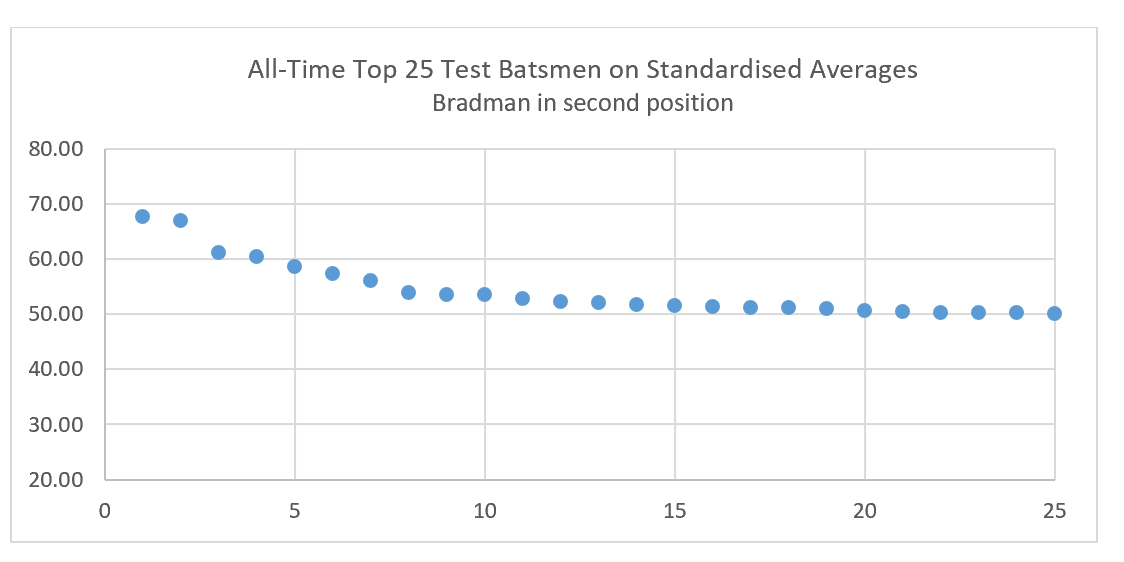
All these twenty-five players have at least 20 innings, except for Barry Richards (7 innings, all completed), Sid Barnes (19, two not outs) and Taslim Arif of Pakistan (10, two not outs).[xx]
The key to appreciating this contrasting picture is that, in physiological terms, Bradman was not outstanding. Most notably, the sharpness of his eyesight and the speed at which his brain registered changes in his field of view (most notably, the ball release from the bowler’s hand) were not above the norm for high performing sportsmen of his time; and being short in height he was at a disadvantage in his reach at the crease. Nor did he benefit materially from having a relatively high proportion of Not Out innings, at 12.5%. The norm for the leading 63 on official averages is 10.6%; applied to Bradman, his average would be 97.8. And of the next six after him, Pollock has the lowest proportion of Not Outs at 9.8%.[xxi]
My finding that the apparent gulf is an illusion is understandable given that Bradman had only a normal physiological foundation to work. It signals that he was human after all! He shares top position due to an uncanny anticipation of a delivery’s path, his finely tuned hand-eye co-ordination and very agile footwork, plus excellent shot selection and placement. All these being allied to an ingrained attacking outlook.
Potential Refinements: A Role for Readers
As with all such exercises, various improvements are possible, albeit usually at the cost of somewhat greater complexity. I invite readers to formulate their own ideas and see what they imply by incorporating them into the basic model or some version of it.
Without wishing to anticipate these ideas, I thought it might be useful to briefly note some of the possible refinements that suggest themselves to the author:
- Focus on completed careers, as a matter of principle, so as to compare players more fully on a like-for-like basis.
- Give a weighting for career length, the counter being that this may simply be valuing doing more or less the same thing the same way for longer, and reflect opportunity as against a lack of it.
- Raise the general qualification from twenty to, say 30 or 40 innings to give a more reliable “take” on relative ability.[xxii]
- Identify those players with a high proportion of Not Out innings that might be distorting (though very few of my 173 exceed 20%).
- Add a premium of around 5 runs to those usually opening the innings, as I have suggested elsewhere, to reflect the comparative difficulty of the role.
[i] The initial exercise is contained in the book Rescuing Don Bradman from Splendid Isolation. Published by PK Associates, Melbourne, February 2019.
[ii] Stephen Jay Gould: The Model Batter, Extinction of 0.400 Hitting and the Improvement in Baseball. Forming Part Three of his book, Life’s Grandeur (Jonathan Cape, London, 1996), pages 77-132.
[iii] For each era, having identified the batsmen with 20 plus innings (eg 476 for the ten main Test countries of the Present Era), those with an average of at least one standard deviation above the Mean value (the overall average) were selected as the leaders for this comparative assessment.
[iv] 19 innings by Sid Barnes, Alan Melville and KS Duleepsinhji; 18 by Vijay Merchant and England’s CAG Russell; 10 by Pakistan’s Taslim Arif; and 7 by Barry Richards.
[v] In cases of a large first innings total where the intention has been to enforce a follow-on (with a lead of at least 200 or 150 for three or four day matches), dead runs are again identified with reference to reasonable expectations at the time as to the opposition’s likely capabilities in responding. The focus is on the prospect of the opposition’s two innings setting up a realistic possibility of it emerging as the winner (as distinct from a remote or negligible possibility).
[vi] A total of 99 timeless Test matches were staged up to WW2, including all those in Australia which were predominantly against England. Dead runs scored in these matches were pointless – without any value – rather than actually being counter-productive. The argument that piling on more runs after the stage when the opposition couldn’t win, and so was doomed to defeat, had value in tiring their bowlers and fielders, and was perhaps also demoralising, holds little water as there was plenty of recovery time between Tests during a Timeless series – typically somewhere between one and a half and three weeks.
[vii] The only comment I could find of Bradman making runs of no value to his Test team is a brief comment by Greg Chappell: “No one would have understood exactly what it was that drove him (Bradman) so relentlessly to make runs far beyond their need on occasions.”
[viii] The lower thresholds specified for the two pre-WW1 eras equates to the lower team dismissal average of each compared with the subsequent six eras taken together.
[ix] Five of the eight Tests that spawned DGB’s dead runs were “timeless” matches, but the effect of his floggings on bowlers wouldn’t have lingered on until the next Test encounter as the gaps between them were 24, 15, 10 and 22 days (the other one was the final match of a Test series).
[x] The highest proportion of dead runs for the 25 batsmen sampled is 4.0%, 4.2% and 5.0%, compared with Bradman’s full tally of 10.1%.
[xi] The standard statistical test indicates that, at a confidence level of 80%, the margin of error is 40.7% up and down on the sample estimate, given the sample size and an assumed standard deviation of the data set of 5.6. (That standard deviation is based on the distribution of the finalised averages, in the absence of a distribution specifically for dead runs.)
[xii] The formula for the standard deviation comprises six (straightforward) steps and gives an answer for the “typical” deviation from the overall average which is somewhat higher than simply taking the arithmetic average of all the absolute differences from the overall average (termed the “Mean Absolute Deviation” – MAD). The procedure involves squaring each of the differences (“variances”) from the overall average, summing the resulting values, then finding the arithmetic average of the variances and, finally, taking the square root of that combined sum. The higher answer than for the MAD comes about by the act of squaring the variances which has the effect of weighting more heavily those variances of a relatively large magnitude. The more unevenly spaced are the individual career averages in the set of data, the greater will be the answer for the standard deviation, even if the highest and lowest values remain unaltered.
For example, in the case of the career averages of the 476 batsmen of the Present Era (with a minimum of twenty innings), the Mean Absolute Deviation works out at 10.98 and the Standard Deviation at 13.25.
The standard deviation method has no inherent advantages over the simpler (MAD) method for the purposes of this exercise (or over taking differences from the median value of the data set). It has been used here as it is the commonly used measure and so facilitates comparisons with the results of other studies of Test batsmen’s dominance, notably those by Stephen Walters done in 2014, and two decades ago by Geoff Dickson and colleagues and by Charles Davis – references given below. (Stephen Walters: Did Don Bradman’s cricketing genius make him a statistical outlier? Significance magazine, Sports section, 3 February 2015.)
[xiii] The spread of these averages comes close to the statistician’s construct of a “normal”, or fully symmetrical, distribution; and on a standard test is only “mildly” skewed in overall terms. 52.1% of the values lie above the Mean value of 27.15 runs while the Median value is close at 27.88 runs. As expected, the averages are somewhat more heavily represented at the bottom end: 12.6% of the values lying in the 1-10 range compared with 4.4% at top end of 50-62.
[xiv] In principle, any era can act as the common one for making the translation of dominance ratings as the ranking of batsmen and the relativities of their standardised averages won’t be affected (only their absolute values would be). The Present Era is the natural one to use due to its familiarity for readers and easily absorbed results.
[xv] When expressed per decade, the rate of batting improvement from 1920 onwards lies between 1.0% and 2.5% (except in one case), averaging out at 1.6% per decade, with a somewhat lower rate applying to the pre-WW1 period at around 0.7% per decade.
[xvi] Once the improvement in expertise has been factored in, new dominance ratings can then be calculated for past batsmen in the context of the Present Era. This implies a rating for Bradman of 2.92, instead of 3.24 for his own playing time. Taking a few others: for Barry Richards, 3.19 becomes 3.06; for Graeme Pollock, 2.16 becomes 2.02; for Gary Sobers, 1.95 becomes 1.80; and for FS Jackson, 2.02 becomes 1.74.
[xvii] G. Dickson and others: A cricketer for the ages: Changes to the performance variation of Test cricket batting from 1877-1997. Paper given at third annual conference of Sport Management Association of Australian and New Zealand, Griffiths University, Gold Coast, Queensland, 1998.
[xviii] The answer to this one is that Viv Richards faced either Roberts, Holding, Croft or Marshall during 35 innings for Somerset and Glamorgan (twice not out), averaging 53.3, this being a little higher than his overall Test average of 50.2.
He was dismissed by one of these four on only eight occasions – one in four and a half innings – for a very similar average (53.9).
So, on this evidence, there’s little reason to think Richard’s Test average would have been materially lowered by facing these luminaries of his own team.
[xix] In his book of year 2000, Charles Davis has estimated that poor pitches in the period 1877-97 served to depress team totals by 24%.
[xx] Taslim Arif’s ten matches came in 1979/80 and 1980/81 when in his mid-twenties. His average of 62.6 was then in the realms unheard of for someone in both wicket-keeper and opening roles. Following a patient 90 on debut against India, against Australia he made 58 and 8, an undefeated 210, and 31 – all when facing Dennis Lillee at his peak.
Arif’s only poor match came in a loss to the West Indies (duck and 18) facing the bowling of Sylvester Clarke, Colin Croft and Malcolm Marshall, in which only Miandad made a fifty for the team. With Pakistan going 1-0 down in the series, he was dropped and, curiously, never invited back. The selectors had blundered. They tried three openers as a replacement for Arif in the next few matches and all failed; it took eight matches before a measure of stability was restored at the top of the order.
[xxi] Headley 10.0%, Sutcliffe 10.7%, Smith 12.4%, Paynter 16.1%, Voges 22.6%.
[xxii] In personal correspondence, the statistician Charles Davis mentioned that in looking at those who had played 100 plus Tests, it usually wasn’t until about 30-35 Tests that the scatter in an individual’s averages resembled the longer term pattern.


Leave a comment